Weighted vs Unweighted average for azimuthal integration

The aim of this tutorial is to investigate the ability to perform unweighted averages during azimuthal integration and validate the result for intensity and uncertainties propagation.

%matplotlib inline
# use `widget` instead of `inline` for better user-exeperience. `inline` allows to store plots into notebooks.
import time
import numpy
from matplotlib.pyplot import subplots
from scipy.stats import chi2 as chi2_dist
import fabio
import pyFAI
from pyFAI.gui import jupyter
from pyFAI.test.utilstest import UtilsTest
from pyFAI.utils.mathutil import rwp
t0 = time.perf_counter()

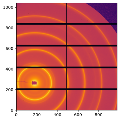
img = fabio.open(UtilsTest.getimage("Pilatus1M.edf")).data
ai = pyFAI.load(UtilsTest.getimage("Pilatus1M.poni"))
print(ai)
jupyter.display(img)

Detector Pilatus 1M	 PixelSize= 172µm, 172µm	 BottomRight (3)
Wavelength= 1.000000 Å
SampleDetDist= 1.583231e+00 m	PONI= 3.341702e-02, 4.122778e-02 m	rot1=0.006487  rot2=0.007558  rot3=0.000000 rad
DirectBeamDist= 1583.310 mm	Center: x=179.981, y=263.859 pix	Tilt= 0.571° tiltPlanRotation= 130.640° λ= 1.000Å

<Axes: >

method = pyFAI.method_registry.IntegrationMethod.parse(("no", "csr", "cython"), dim=1)
weighted = method
unweighted = method.unweighted

#Note
weighted.weighted_average, unweighted.weighted_average, weighted == unweighted

(True, False, True)

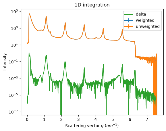
res_w = ai.integrate1d(img, 1000, method=weighted, error_model="poisson", polarization_factor=0.99)
res_u = ai.integrate1d(img, 1000, method=unweighted, error_model="poisson", polarization_factor=0.99)

rwp(res_u, res_w)

np.float64(0.002684804600489726)

ax = jupyter.plot1d(res_w, label="weighted")
ax = jupyter.plot1d(res_u, label="unweighted", ax=ax)
ax.plot(res_w.radial, abs(res_w.intensity-res_u.intensity), label="delta")
ax.legend()
ax.set_yscale("log")

About statistics

Work on a dataset with 1000 frames in a WAXS like configuration

ai_init = {"dist":0.1, 
           "poni1":0.1, 
           "poni2":0.1, 
           "rot1":0.0,
           "rot2":0.0,
           "rot3":0.0,
           "detector": "Pilatus1M", 
           "wavelength":1e-10}
ai = pyFAI.load(ai_init)
unit = pyFAI.units.to_unit("q_A^-1")
detector = ai.detector
npt = 1000 
nimg = 1000
wl = 1e-10
I0 = 1e4
polarization = 0.99
kwargs = {"npt":npt, 
         "polarization_factor": polarization,
         "safe":False,
         "error_model": pyFAI.containers.ErrorModel.POISSON}

print(ai)          

Detector Pilatus 1M	 PixelSize= 172µm, 172µm	 BottomRight (3)
Wavelength= 1.000000 Å
SampleDetDist= 1.000000e-01 m	PONI= 1.000000e-01, 1.000000e-01 m	rot1=0.000000  rot2=0.000000  rot3=0.000000 rad
DirectBeamDist= 100.000 mm	Center: x=581.395, y=581.395 pix	Tilt= 0.000° tiltPlanRotation= 0.000° λ= 1.000Å

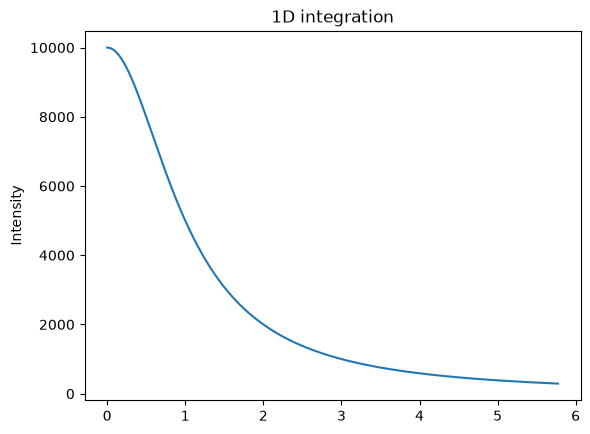
# Generation of a "SAXS-like" curve with the shape of a lorentzian curve
flat = numpy.random.random(detector.shape) + 0.5

qmax = ai.integrate1d(flat, method=method, **kwargs).radial.max()
q = numpy.linspace(0, ai.array_from_unit(unit="q_A^-1").max(), npt)
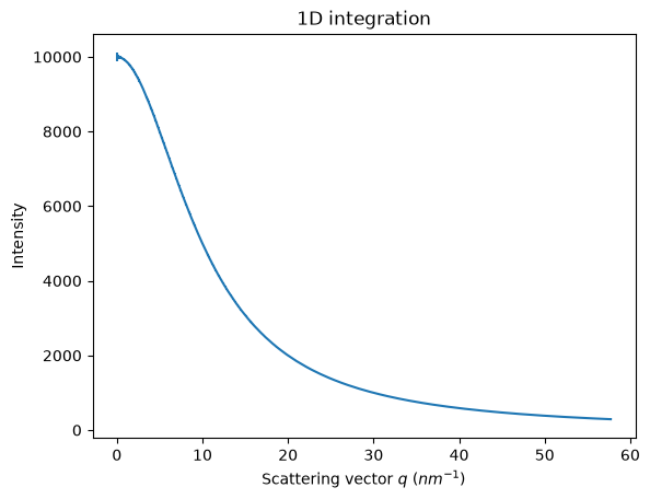
I = I0/(1+q**2)
jupyter.plot1d((q,I))
pass

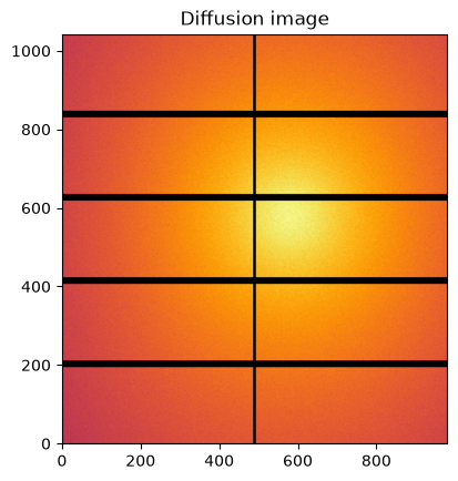
#Reconstruction of diffusion image:

img_theo = ai.calcfrom1d(q, I, dim1_unit=unit, 
                         correctSolidAngle=True,
                         flat=flat,
                         polarization_factor=polarization,
                         mask=ai.detector.mask)
kwargs["flat"] = flat

jupyter.display(img_theo, label="Diffusion image")
pass

res_theo = ai.integrate1d(img_theo, method=method, **kwargs)
jupyter.plot1d(res_theo)

<Axes: title={'center': '1D integration'}, xlabel='Scattering vector $q$ ($nm^{-1}$)', ylabel='Intensity'>

%%time
if "dataset" not in dir():
    dataset = numpy.random.poisson(img_theo, (nimg,) + img_theo.shape)
# else avoid wasting time
print(dataset.nbytes/(1<<20), "MBytes", dataset.shape)

7806.266784667969 MBytes (1000, 1043, 981)
CPU times: user 41.2 s, sys: 1.18 s, total: 42.4 s
Wall time: 42.4 s

res_weighted = ai.integrate1d(dataset[0], method=weighted, **kwargs)
res_unweighted = ai.integrate1d(dataset[0], method=unweighted, **kwargs)
                              
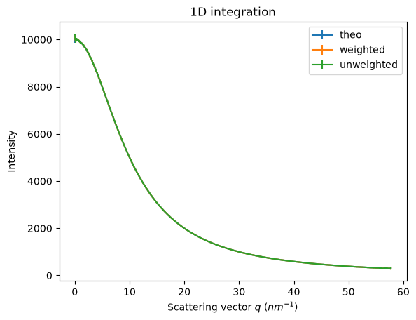
ax = jupyter.plot1d(res_theo, label="theo")
ax = jupyter.plot1d(res_weighted, label="weighted", ax=ax)
ax = jupyter.plot1d(res_unweighted, label="unweighted", ax=ax);

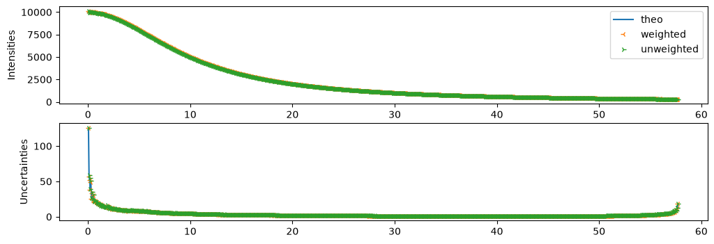
fix,ax = subplots(2, figsize=(12,4))
ax[0].plot(res_theo.radial, res_theo.intensity, label="theo")
ax[1].plot(res_theo.radial, res_theo.sigma, label="theo")
ax[0].plot(res_weighted.radial, res_weighted.intensity, "3", label="weighted")
ax[1].plot(res_weighted.radial, res_weighted.sigma, "3",label="weighted")
ax[0].plot(res_unweighted.radial, res_unweighted.intensity, "4", label="unweighted")
ax[1].plot(res_unweighted.radial, res_unweighted.sigma, "4", label="unweighted")
ax[0].set_ylabel("Intensities")
ax[1].set_ylabel("Uncertainties")
ax[0].legend();

print("Number of paires of images: ", nimg*(nimg-1)//2)

Number of paires of images:  499500

def chi2_curves(res1, res2):
    """Calculate the Chi² value for a pair of integrated data"""
    I = res1.intensity
    J = res2.intensity
    l = len(I)
    assert len(J) == l
    sigma_I = res1.sigma
    sigma_J = res2.sigma
    return ((I-J)**2/(sigma_I**2+sigma_J**2)).sum()/(l-1)

def plot_distribution(ai, kwargs, nbins=100, method=method, ax=None):
    ai.reset()
    results = []
    c2 = []
    integrate = ai.integrate1d
    for i in range(nimg):
        data = dataset[i, :, :]
        r = integrate(data, method=method, **kwargs)
        results.append(r)    
        for j in results[:i]:
            c2.append(chi2_curves(r, j))
    c2 = numpy.array(c2)
    if ax is None:
        fig, ax = subplots()
    h,b,_ = ax.hist(c2, nbins, label="Measured histogram")
    y_sim = chi2_dist.pdf(b*(npt-1), npt)
    y_sim *= h.sum()/y_sim.sum()
    ax.plot(b, y_sim, label=r"$\chi^{2}$ distribution")
    ax.set_title(f"Integrated curves with {integrate.__name__}")
    ax.set_xlabel(r"$\chi^{2}$ values (histogrammed)")
    ax.set_ylabel("Number of occurences")
    ax.legend()
    return ax

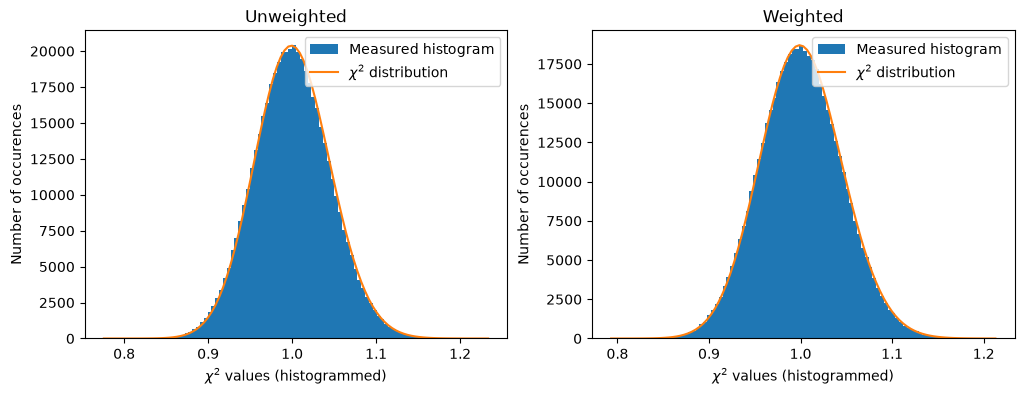
fig,ax = subplots(1,2, figsize=(12,4))
a=plot_distribution(ai, kwargs, method=unweighted, ax=ax[0])
a.set_title("Unweighted")
a=plot_distribution(ai, kwargs, method=weighted, ax=ax[1])
a.set_title("Weighted")

Text(0.5, 1.0, 'Weighted')

print(rwp(ai.integrate1d(dataset[100], method=weighted, **kwargs),
          ai.integrate1d(dataset[100], method=unweighted, **kwargs)))

0.038747450593776774

print(f"Total run-time: {time.perf_counter()-t0:.3f}s")

Total run-time: 90.932s

Conclusion

The two algorithms provide similar results but not strictly the same. The difference is largely beyond the numerical noise since the Rwp between two results is in the range of a few percent. Their performances for the speed is also equivalent. Their results are different but on a statistical point of view, it is difficult to distinguish them.

To me (J. Kieffer, author of pyFAI), the question of the best algorithm remains open.