Inpainting missing data

Missing data in an image can be an issue, especially when one wants to perform Fourier analysis. This tutorial explains how to fill-up missing pixels with values which looks “realistic” and introduce as little perturbation as possible for subsequent analysis. The user should keep the mask nearby and only consider the values of actual pixels and never the one inpainted.

This tutorial will use fully synthetic data to allow comparison between actual (synthetic) data with inpainted values.

The first part of the tutorial is about the generation of a challenging 2D diffraction image with realistic noise and to describe the metric used, then comes the actual tutorial on how to use the inpainting. Finally a benchmark is used based on the metric determined.

Creation of the image

A realistic challenging image should contain:

• Bragg peak rings. We chose LaB6 as guinea-pig, with very sharp peaks, at the limit of the resolution of the detector

• Some amorphous content

• strong polarization effect

• Poissonian noise

One image will be generated but then multiple ones with different noise to discriminate the effect of the noise from other effects.

%matplotlib inline
# Used for documentation to inline plots into notebook
# %matplotlib widget
# uncomment the later for better UI
from matplotlib.pyplot import subplots
import numpy

import pyFAI
print("Using pyFAI version: ", pyFAI.version)
from pyFAI.gui import jupyter
import pyFAI.test.utilstest
from pyFAI.calibrant import get_calibrant
import time
start_time = time.perf_counter()

Using pyFAI version:  2026.6.0-dev0

detector = pyFAI.detector_factory("Pilatus2MCdTe")
mask = detector.mask.copy()
nomask = numpy.zeros_like(mask)
detector.mask=nomask
ai = pyFAI.load({"detector":detector})
ai.setFit2D(200, 200, 200)
ai.wavelength = 3e-11
print(ai)

Detector Pilatus CdTe 2M	 PixelSize= 172µm, 172µm	 BottomRight (3)
Wavelength= 0.300000 Å
SampleDetDist= 2.000000e-01 m	PONI= 3.440000e-02, 3.440000e-02 m	rot1=0.000000  rot2=0.000000  rot3=0.000000 rad
DirectBeamDist= 200.000 mm	Center: x=200.000, y=200.000 pix	Tilt= 0.000° tiltPlanRotation= 0.000° λ= 0.300Å

LaB6 = get_calibrant("LaB6")
LaB6.wavelength = ai.wavelength
print(LaB6)
r = ai.array_from_unit(unit="q_nm^-1")
decay_b = numpy.exp(-(r-50)**2/2000)
bragg = LaB6.fake_calibration_image(ai, Imax=1e4, resolution=0.1) * ai.polarization(factor=1.0) * decay_b
decay_a = numpy.exp(-r/100)
amorphous = 1000*ai.polarization(factor=1.0)*ai.solidAngleArray() * decay_a
img_nomask = bragg + amorphous
#Not the same noise function for all images two images
img_nomask1 = numpy.random.poisson(img_nomask)
img_nomask2 = numpy.random.poisson(img_nomask)
img = numpy.random.poisson(img_nomask)
img[numpy.where(mask)] = -1
fig,ax = subplots(1,2, figsize=(10,5))
jupyter.display(img=img, label="With mask", ax=ax[0])
jupyter.display(img=img_nomask, label="Without mask", ax=ax[1]);

LaB6 Calibrant with 640 reflections at wavelength 3e-11

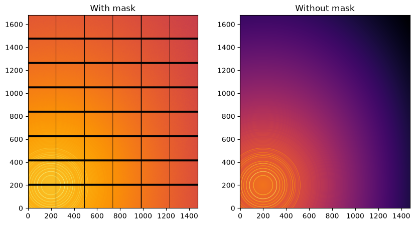
Note the aliasing effect on the displayed images.

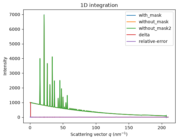
We will measure now the effect after 1D integration. We do not correct for polarization on purpose to highlight the defect one wishes to wipe out. We use a R-factor to describe the quality of the 1D-integrated signal.

kwargs = {"npt":2000, "unit":"q_nm^-1", "method":("full", "histogram", "cython"), "radial_range":(0,210)}
wo = ai.integrate1d(img_nomask, **kwargs)
wo2 = ai.integrate1d(img_nomask2, **kwargs)
wm = ai.integrate1d(img, mask=mask, **kwargs)
ax = jupyter.plot1d(wm , label="with_mask")
ax.plot(*wo, label="without_mask")
ax.plot(*wo2, label="without_mask2")
ax.plot(wo.radial, wo.intensity-wm.intensity, label="delta")
ax.plot(wo.radial, wo.intensity-wo2.intensity, label="relative-error")
ax.legend()
print("Between masked and non masked image R= %s"%pyFAI.utils.mathutil.rwp(wm,wo))
print("Between two different non-masked images R'= %s"%pyFAI.utils.mathutil.rwp(wo2,wo))

Between masked and non masked image R= 5.674154439359792
Between two different non-masked images R'= 0.462136015724442

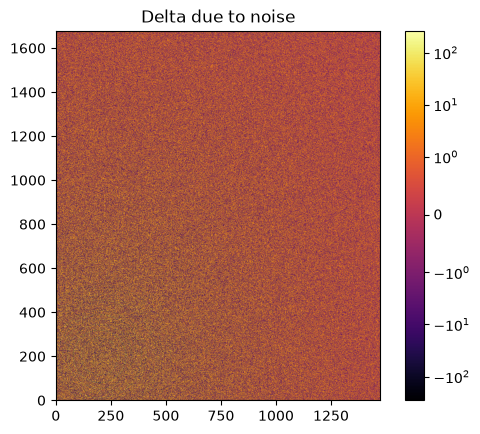
# Effect of the noise on the delta image
fig, ax = subplots()
jupyter.display(img=img_nomask-img_nomask2, label="Delta due to noise", ax=ax)
ax.figure.colorbar(ax.images[0])

<matplotlib.colorbar.Colorbar at 0x7f58a0123230>

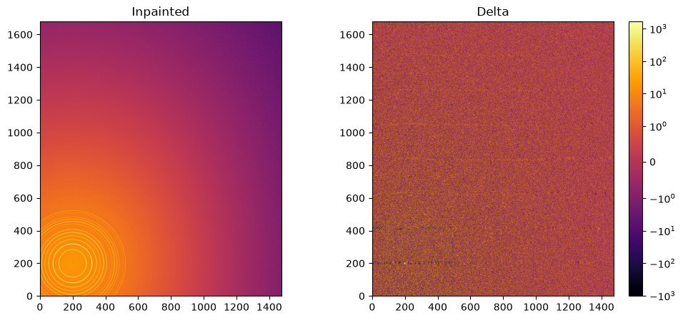
Inpainting

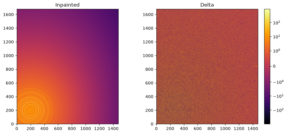
This part describes how to paint the missing pixels for having a “natural-looking image”. The delta image contains the difference with the original image

#Inpainting:
inpainted = ai.inpainting(img, mask=mask, 
                          method=("no", "histogram", "cython"),
                          poissonian=True, grow_mask=3)
fig, ax = subplots(1, 2, figsize=(12,5))
jupyter.display(img=inpainted, label="Inpainted", ax=ax[0])
jupyter.display(img=img_nomask-inpainted, label="Delta", ax=ax[1])
ax[1].figure.colorbar(ax[1].images[0]);

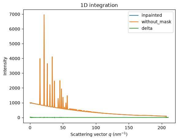
# Comparison of the inpained image with the original one:
wm = ai.integrate1d(inpainted, **kwargs)
wo = ai.integrate1d(img_nomask, **kwargs)
ax = jupyter.plot1d(wm , label="inpainted")
ax.plot(*wo, label="without_mask")
ax.plot(wo.radial, wo.intensity-wm.intensity, label="delta")
ax.legend()
print("R= %s"%pyFAI.utils.mathutil.rwp(wm,wo))

R= 0.6445549231619412

One can see by zooming in that the main effect on inpainting is a broadening of the signal in the inpainted region. This could (partially) be addressed by increasing the number of radial bins used in the inpainting.

Benchmarking and optimization of the parameters

The parameter set depends on the detector, the experiment geometry and the type of signal on the detector. Finer detail require finer slicing.

#Basic benchmarking of execution time for default options:
%timeit inpainted = ai.inpainting(img, mask=mask)

123 ms ± 9.18 ms per loop (mean ± std. dev. of 7 runs, 1 loop each)

wo = ai.integrate1d(img_nomask, **kwargs)
R_best = numpy.finfo("float32").max
best = {}
for m in (("no", "csc", "cython"), ("bbox", "csc","cython"), ("full", "csc","cython")):
    for k in (512, 1024, 2048, 4096):
        ai.reset()
        for i in (0, 1, 2, 4, 8):
            inpainted = ai.inpainting(img, mask=mask, poissonian=True, method=m, npt_rad=k, grow_mask=i)
            wm = ai.integrate1d(inpainted, **kwargs)
            R = pyFAI.utils.mathutil.rwp(wm,wo)
            if R<R_best:
                R_best = R
                best={"method":m,
                      "npt_rad":k, 
                      "grow_mask":i}
            print(f"method: {m} npt_rad={k} grow={i}; R= {R:.3f}")
print("Best configuration:", best)

method: ('no', 'csc', 'cython') npt_rad=512 grow=0; R= 2.267

method: ('no', 'csc', 'cython') npt_rad=512 grow=1; R= 0.808

method: ('no', 'csc', 'cython') npt_rad=512 grow=2; R= 0.514

method: ('no', 'csc', 'cython') npt_rad=512 grow=4; R= 0.482

method: ('no', 'csc', 'cython') npt_rad=512 grow=8; R= 0.455

method: ('no', 'csc', 'cython') npt_rad=1024 grow=0; R= 2.458

method: ('no', 'csc', 'cython') npt_rad=1024 grow=1; R= 0.878

method: ('no', 'csc', 'cython') npt_rad=1024 grow=2; R= 0.699

method: ('no', 'csc', 'cython') npt_rad=1024 grow=4; R= 0.616

method: ('no', 'csc', 'cython') npt_rad=1024 grow=8; R= 0.340

method: ('no', 'csc', 'cython') npt_rad=2048 grow=0; R= 2.753

method: ('no', 'csc', 'cython') npt_rad=2048 grow=1; R= 1.162

method: ('no', 'csc', 'cython') npt_rad=2048 grow=2; R= 1.066

method: ('no', 'csc', 'cython') npt_rad=2048 grow=4; R= 0.935

method: ('no', 'csc', 'cython') npt_rad=2048 grow=8; R= 0.688

method: ('no', 'csc', 'cython') npt_rad=4096 grow=0; R= 2.683

method: ('no', 'csc', 'cython') npt_rad=4096 grow=1; R= 1.202

method: ('no', 'csc', 'cython') npt_rad=4096 grow=2; R= 1.188

method: ('no', 'csc', 'cython') npt_rad=4096 grow=4; R= 1.131

method: ('no', 'csc', 'cython') npt_rad=4096 grow=8; R= 1.007

method: ('bbox', 'csc', 'cython') npt_rad=512 grow=0; R= 0.504

method: ('bbox', 'csc', 'cython') npt_rad=512 grow=1; R= 0.477

method: ('bbox', 'csc', 'cython') npt_rad=512 grow=2; R= 0.471

method: ('bbox', 'csc', 'cython') npt_rad=512 grow=4; R= 0.452

method: ('bbox', 'csc', 'cython') npt_rad=512 grow=8; R= 0.454

method: ('bbox', 'csc', 'cython') npt_rad=1024 grow=0; R= 0.346

method: ('bbox', 'csc', 'cython') npt_rad=1024 grow=1; R= 0.321

method: ('bbox', 'csc', 'cython') npt_rad=1024 grow=2; R= 0.317

method: ('bbox', 'csc', 'cython') npt_rad=1024 grow=4; R= 0.312

method: ('bbox', 'csc', 'cython') npt_rad=1024 grow=8; R= 0.308

method: ('bbox', 'csc', 'cython') npt_rad=2048 grow=0; R= 0.284

method: ('bbox', 'csc', 'cython') npt_rad=2048 grow=1; R= 0.279

method: ('bbox', 'csc', 'cython') npt_rad=2048 grow=2; R= 0.273

method: ('bbox', 'csc', 'cython') npt_rad=2048 grow=4; R= 0.270

method: ('bbox', 'csc', 'cython') npt_rad=2048 grow=8; R= 0.275

method: ('bbox', 'csc', 'cython') npt_rad=4096 grow=0; R= 0.268

method: ('bbox', 'csc', 'cython') npt_rad=4096 grow=1; R= 0.262

method: ('bbox', 'csc', 'cython') npt_rad=4096 grow=2; R= 0.267

method: ('bbox', 'csc', 'cython') npt_rad=4096 grow=4; R= 0.265

method: ('bbox', 'csc', 'cython') npt_rad=4096 grow=8; R= 0.271

method: ('full', 'csc', 'cython') npt_rad=512 grow=0; R= 0.517

method: ('full', 'csc', 'cython') npt_rad=512 grow=1; R= 0.462

method: ('full', 'csc', 'cython') npt_rad=512 grow=2; R= 0.456

method: ('full', 'csc', 'cython') npt_rad=512 grow=4; R= 0.456

method: ('full', 'csc', 'cython') npt_rad=512 grow=8; R= 0.454

method: ('full', 'csc', 'cython') npt_rad=1024 grow=0; R= 0.336

method: ('full', 'csc', 'cython') npt_rad=1024 grow=1; R= 0.316

method: ('full', 'csc', 'cython') npt_rad=1024 grow=2; R= 0.316

method: ('full', 'csc', 'cython') npt_rad=1024 grow=4; R= 0.322

method: ('full', 'csc', 'cython') npt_rad=1024 grow=8; R= 0.309

method: ('full', 'csc', 'cython') npt_rad=2048 grow=0; R= 1.122

method: ('full', 'csc', 'cython') npt_rad=2048 grow=1; R= 1.141

method: ('full', 'csc', 'cython') npt_rad=2048 grow=2; R= 0.911

method: ('full', 'csc', 'cython') npt_rad=2048 grow=4; R= 0.738

method: ('full', 'csc', 'cython') npt_rad=2048 grow=8; R= 0.733

method: ('full', 'csc', 'cython') npt_rad=4096 grow=0; R= 0.938

method: ('full', 'csc', 'cython') npt_rad=4096 grow=1; R= 0.960

method: ('full', 'csc', 'cython') npt_rad=4096 grow=2; R= 0.962

method: ('full', 'csc', 'cython') npt_rad=4096 grow=4; R= 0.927

method: ('full', 'csc', 'cython') npt_rad=4096 grow=8; R= 0.709
Best configuration: {'method': ('bbox', 'csc', 'cython'), 'npt_rad': 4096, 'grow_mask': 1}

#Inpainting, best solution found:
ai.reset()
%time inpainted = ai.inpainting(img, mask=mask, poissonian=True, **best)
fig, ax = subplots(1, 2, figsize=(12, 5))
jupyter.display(img=inpainted, label="Inpainted", ax=ax[0])
jupyter.display(img=img_nomask-inpainted, label="Delta", ax=ax[1])
ax[1].figure.colorbar(ax[1].images[0]);

CPU times: user 3.2 s, sys: 81.6 ms, total: 3.28 s
Wall time: 1.41 s

# Comparison of the inpained image with the original one:
wm = ai.integrate1d(inpainted, **kwargs)
wo = ai.integrate1d(img_nomask, **kwargs)
ax = jupyter.plot1d(wm , label="inpainted")
ax.plot(*wo, label="without_mask")
ax.plot(wo.radial, wo.intensity-wm.intensity, label="delta")
ax.legend()
print("R= %s"%pyFAI.utils.mathutil.rwp(wm,wo))

R= 0.26093294473008155

Conclusion

Inpainting is one of the only solutions to fill up the gaps in the detector when Fourier analysis is needed. This tutorial explains basically how this is possible using the pyFAI library and how to optimize the parameter set for inpainting. The result may greatly vary with detector position and tilt and the kind of signal (amorphous or more spotty).

print(f"Execution time: {time.perf_counter()-start_time:.3f} s")

Execution time: 64.213 s