Demo of usage of the MultiGeometry class of pyFAI#
For this tutorial, we will use the Jupyter notebook, formerly known as IPython, and take advantage of the integration of matplotlib.
%matplotlib inline
# use `widget` for better user experience; `inline` is for documentation generation

import time
start_time = time.perf_counter()

import numpy
from matplotlib.pyplot import subplots

import pyFAI
from pyFAI.method_registry import IntegrationMethod
from pyFAI.gui import jupyter
print("Using pyFAI verison: ", pyFAI.version)
Using pyFAI verison: 2026.6.0-dev0
The multi_geometry module of pyFAI allows you to integrate multiple images taken at various image positions, all together. This tutorial will explain you how to perform azimuthal integration in three use-cases: translation of the detector, rotation of the detector around the sample and finally how to fill gaps of a pixel detector. But before, we need to know how to generate fake diffraction images.
Generation of diffraction images#
pyFAI supports approximately 20 different reference samples known as calibrants. We will use them to generate fake diffraction images knowing the detector and its position in space
import pyFAI.calibrant
print("Number of known calibrants: %s"%len(pyFAI.calibrant.ALL_CALIBRANTS))
print(", ".join(pyFAI.calibrant.ALL_CALIBRANTS.keys()))
Number of known calibrants: 39
Si_SRM640e, Si_SRM640, alpha_Al2O3_SRM676a_2008, Si_SRM640d, AgBh, cristobaltite, C14H30O, Au, LaB6_SRM660b, Pt, Si_SRM640c, mock, TiO2, diamond, NaCl, alpha_Al2O3, CrOx, Si_SRM640b, alpha_Al2O3_SRM676, hydrocerussite, alpha_Al2O3_SRM676a_2015, CuO, LaB6, Ni, Cr2O3, ZnO, Si, CeO2, Al, verneite, LaB6_SRM660a, LaB6_SRM660c, quartz, C60, PBBA, vanadinite, lysozyme, Si_SRM640a, graphite
wavelength = 1e-10  # m
LaB6 = pyFAI.calibrant.get_calibrant("LaB6")
LaB6.wavelength = wavelength
print(LaB6)
print("Number of reflections for calibrant at given wavelength: %i"%len(LaB6.dspacing))
LaB6 Calibrant with 59 reflections at wavelength 1e-10
Number of reflections for calibrant at given wavelength: 59
We will start with a “simple” detector called Titan (built by Oxford Diffraction but now sold by Agilent). It is a CCD detector with scintillator and magnifying optics fibers. The pixel size is constant: 60µm
import pyFAI.detectors
det = pyFAI.detectors.Titan()
print(det)
p1, p2, p3 = det.calc_cartesian_positions()
print("Detector is flat, P3= %s"%p3)
poni1 = p1.mean()
poni2 = p2.mean()
print("Center of the detector: poni1=%s poni2=%s"%(poni1, poni2))
Detector Titan 2k x 2k	 PixelSize= 60µm, 60µm	 BottomRight (3)
Detector is flat, P3= None
Center of the detector: poni1=0.06144 poni2=0.06144
The detector is placed orthogonal to the beam at 10cm. This geometry is saved into an AzimuthalIntegrator instance:
ai = pyFAI.load({"dist":0.1, "poni1":poni1, "poni2":poni2, "detector":det, "wavelength":wavelength})
print(ai)

#Selection of the methods for integrating
method = IntegrationMethod.parse("full", dim=1)
method2d = IntegrationMethod.select_one_available(("pseudo","histogram","cython"), dim=2)

print(f"Integration method in 1d: {method}\nIntegration method in 2d: {method2d}")
Detector Titan 2k x 2k	 PixelSize= 60µm, 60µm	 BottomRight (3)
Wavelength= 1.000000 Å
SampleDetDist= 1.000000e-01 m	PONI= 6.144000e-02, 6.144000e-02 m	rot1=0.000000  rot2=0.000000  rot3=0.000000 rad
DirectBeamDist= 100.000 mm	Center: x=1024.000, y=1024.000 pix	Tilt= 0.000° tiltPlanRotation= 0.000° λ= 1.000Å
Integration method in 1d: IntegrationMethod(1d int, full split, histogram, cython)
Integration method in 2d: IntegrationMethod(2d int, pseudo split, histogram, cython)
With the calibrant, wavelength, detector, and geometry defined, one can simulate the 2D diffraction pattern:
img = LaB6.fake_calibration_image(ai)
jupyter.display(img, label="Simulated LaB6");
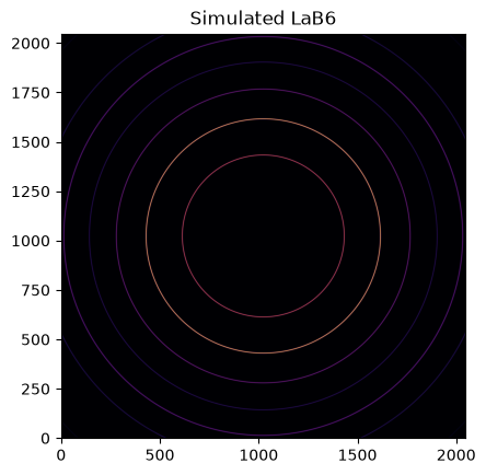
This image can be integrated in q-space and plotted:
jupyter.plot1d(ai.integrate1d(img, 1000, method=method));
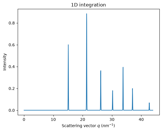
Note: pyFAI does know about the ring position but nothing about relative intensities of rings.
Translation of the detector along the vertical axis#
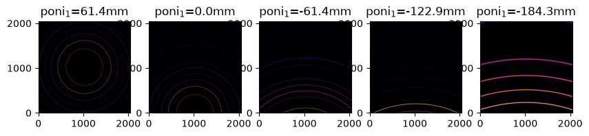
The vertical axis is defined along the poni1. If one moves the detector higher, the poni will appear at lower coordinates. So let’s define 5 upwards vertical translations of half the detector size.
For this we will duplicate 5x the AzimuthalIntegrator object, but instances of AzimuthalIntegrator are mutable, so it is important to create an actual copy and not a view on them. In Python, one can use the copy function of the copy module:
import copy
We will now offset the poni1 value of each AzimuthalIntegrator, which corresponds to a vertical translation. Each subsequent image is offset by half a detector width (stored as poni1).
ais = []
imgs = []
fig, ax = subplots(1,5, figsize=(10,2))
for i in range(5):
    my_ai = copy.deepcopy(ai)
    my_ai.poni1 -= i*poni1
    my_img = LaB6.fake_calibration_image(my_ai)
    jupyter.display(my_img, label="poni$_1$=%3.1fmm"%(1e3*my_ai.poni1), ax=ax[i])
    ais.append(my_ai)
    imgs.append(my_img)
    print(my_ai)
Detector Titan 2k x 2k	 PixelSize= 60µm, 60µm	 BottomRight (3)
Wavelength= 1.000000 Å
SampleDetDist= 1.000000e-01 m	PONI= 6.144000e-02, 6.144000e-02 m	rot1=0.000000  rot2=0.000000  rot3=0.000000 rad
DirectBeamDist= 100.000 mm	Center: x=1024.000, y=1024.000 pix	Tilt= 0.000° tiltPlanRotation= 0.000° λ= 1.000Å
Detector Titan 2k x 2k	 PixelSize= 60µm, 60µm	 BottomRight (3)
Wavelength= 1.000000 Å
SampleDetDist= 1.000000e-01 m	PONI= 0.000000e+00, 6.144000e-02 m	rot1=0.000000  rot2=0.000000  rot3=0.000000 rad
DirectBeamDist= 100.000 mm	Center: x=1024.000, y=0.000 pix	Tilt= 0.000° tiltPlanRotation= 0.000° λ= 1.000Å
Detector Titan 2k x 2k	 PixelSize= 60µm, 60µm	 BottomRight (3)
Wavelength= 1.000000 Å
SampleDetDist= 1.000000e-01 m	PONI= -6.144000e-02, 6.144000e-02 m	rot1=0.000000  rot2=0.000000  rot3=0.000000 rad
DirectBeamDist= 100.000 mm	Center: x=1024.000, y=-1024.000 pix	Tilt= 0.000° tiltPlanRotation= 0.000° λ= 1.000Å
Detector Titan 2k x 2k	 PixelSize= 60µm, 60µm	 BottomRight (3)
Wavelength= 1.000000 Å
SampleDetDist= 1.000000e-01 m	PONI= -1.228800e-01, 6.144000e-02 m	rot1=0.000000  rot2=0.000000  rot3=0.000000 rad
DirectBeamDist= 100.000 mm	Center: x=1024.000, y=-2048.000 pix	Tilt= 0.000° tiltPlanRotation= 0.000° λ= 1.000Å
Detector Titan 2k x 2k	 PixelSize= 60µm, 60µm	 BottomRight (3)
Wavelength= 1.000000 Å
SampleDetDist= 1.000000e-01 m	PONI= -1.843200e-01, 6.144000e-02 m	rot1=0.000000  rot2=0.000000  rot3=0.000000 rad
DirectBeamDist= 100.000 mm	Center: x=1024.000, y=-3072.000 pix	Tilt= 0.000° tiltPlanRotation= 0.000° λ= 1.000Å
MultiGeometry integrator#
The MultiGeometry instance can be created from any list of AzimuthalIntegrator instances or list of poni-files. Here we will use the former method.
The main difference of a MultiIntegrator with a “normal” AzimuthalIntegrator comes from the definition of the output space in the constructor of the object. One needs to specify the unit and the integration range.
from pyFAI.multi_geometry import MultiGeometry
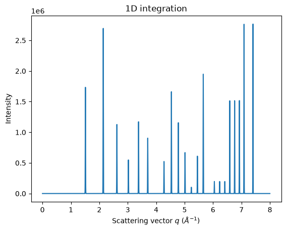
mg = MultiGeometry(ais, unit="q_A^-1", radial_range=(0, 8))
print(mg)
MultiGeometry integrator with 5 geometries on (0, 8) radial range ((q_A^-1, chi_deg)) and None azimuthal range (deg)
MultiGeometry integrators can be used in a similar way to “normal” AzimuthalIntegrators. Keep in mind that the output intensity is always scaled to absolute solid angle.
ax = jupyter.plot1d(mg.integrate1d(imgs, 10000, method=method));
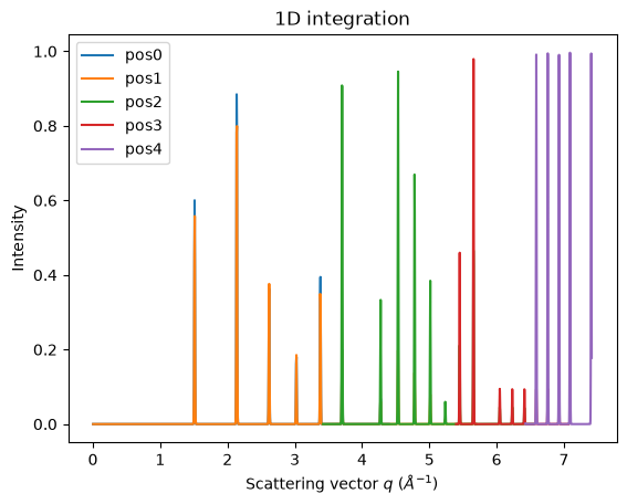
fig, ax = subplots()
for idx, (i, a)  in enumerate(zip(imgs, ais)):
    jupyter.plot1d(a.integrate1d(i, 1000, unit="q_A^-1", method=method), label="pos%i"%idx, ax=ax)
Rotation of the detector#
The advantage of translating the detector is that it simulates a larger detector. However, this approach quickly reaches its limit: as the detector height increases, the solid angle decreases, inducing artificial noise. One solution is to keep the detector at a constant distance and rotate it instead.
This setup is common when mounting a detector on a goniometer.
Creation of diffraction images#
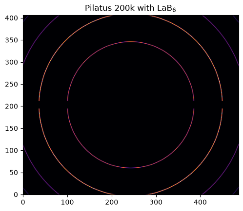
In this example, we will use a Pilatus 200k with two modules. It has a gap between the two detectors and we will see how the MultiGeometry can help.
As previously, we will use LaB6 but instead of translating the images, we will rotate them along the second axis:
det = pyFAI.detectors.detector_factory("pilatus200k")
p1, p2, p3 = det.calc_cartesian_positions()
print(p3)
poni1 = p1.mean()
poni2 = p2.mean()
print(poni1)
print(poni2)
None
0.035002
0.041881997
ai = pyFAI.load({"dist":0.1, "poni1":poni1, "poni2":poni2, "detector":det})
img = LaB6.fake_calibration_image(ai)

jupyter.display(img, label="Pilatus 200k with LaB$_6$");
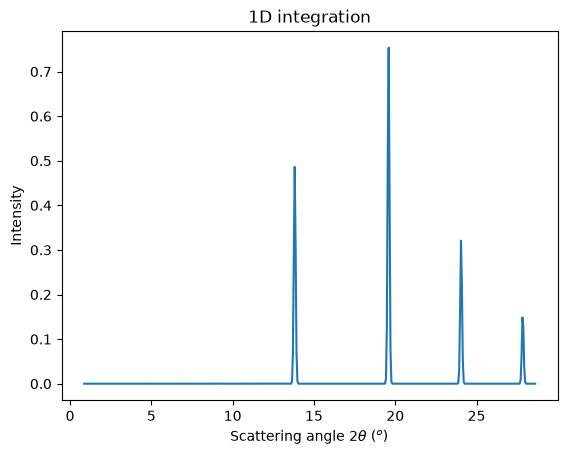
jupyter.plot1d(ai.integrate1d(img, 500, unit="2th_deg", method=method));
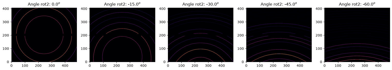
We will rotate the detector with a step size of 15 degrees.
step = 15*numpy.pi/180
ais = []
imgs = []
fig, ax = subplots(1, 5, figsize=(20,4))
for i in range(5):
    my_ai = copy.deepcopy(ai)
    my_ai.rot2 -= i*step
    my_img = LaB6.fake_calibration_image(my_ai)
    jupyter.display(my_img, label="Angle rot2: %.1f$^o$"%numpy.degrees(my_ai.rot2), ax=ax[i])
    ais.append(my_ai)
    imgs.append(my_img)
    print(my_ai)
Detector Pilatus 200k	 PixelSize= 172µm, 172µm	 BottomRight (3)
SampleDetDist= 1.000000e-01 m	PONI= 3.500200e-02, 4.188200e-02 m	rot1=0.000000  rot2=0.000000  rot3=0.000000 rad
DirectBeamDist= 100.000 mm	Center: x=243.500, y=203.500 pix	Tilt= 0.000° tiltPlanRotation= 0.000°
Detector Pilatus 200k	 PixelSize= 172µm, 172µm	 BottomRight (3)
SampleDetDist= 1.000000e-01 m	PONI= 3.500200e-02, 4.188200e-02 m	rot1=0.000000  rot2=-0.261799  rot3=0.000000 rad
DirectBeamDist= 103.528 mm	Center: x=243.500, y=47.716 pix	Tilt= 15.000° tiltPlanRotation= -90.000°
Detector Pilatus 200k	 PixelSize= 172µm, 172µm	 BottomRight (3)
SampleDetDist= 1.000000e-01 m	PONI= 3.500200e-02, 4.188200e-02 m	rot1=0.000000  rot2=-0.523599  rot3=0.000000 rad
DirectBeamDist= 115.470 mm	Center: x=243.500, y=-132.169 pix	Tilt= 30.000° tiltPlanRotation= -90.000°
Detector Pilatus 200k	 PixelSize= 172µm, 172µm	 BottomRight (3)
SampleDetDist= 1.000000e-01 m	PONI= 3.500200e-02, 4.188200e-02 m	rot1=0.000000  rot2=-0.785398  rot3=0.000000 rad
DirectBeamDist= 141.421 mm	Center: x=243.500, y=-377.895 pix	Tilt= 45.000° tiltPlanRotation= -90.000°
Detector Pilatus 200k	 PixelSize= 172µm, 172µm	 BottomRight (3)
SampleDetDist= 1.000000e-01 m	PONI= 3.500200e-02, 4.188200e-02 m	rot1=0.000000  rot2=-1.047198  rot3=0.000000 rad
DirectBeamDist= 200.000 mm	Center: x=243.500, y=-803.506 pix	Tilt= 60.000° tiltPlanRotation= -90.000°
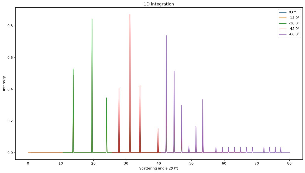
fig, ax = subplots(figsize=(15,8))
for i, a in zip(imgs, ais):
    jupyter.plot1d(a.integrate1d(i, 1000, unit="2th_deg", method=method),
                   label="%.1f$^o$"%numpy.degrees(a.rot2), ax=ax);
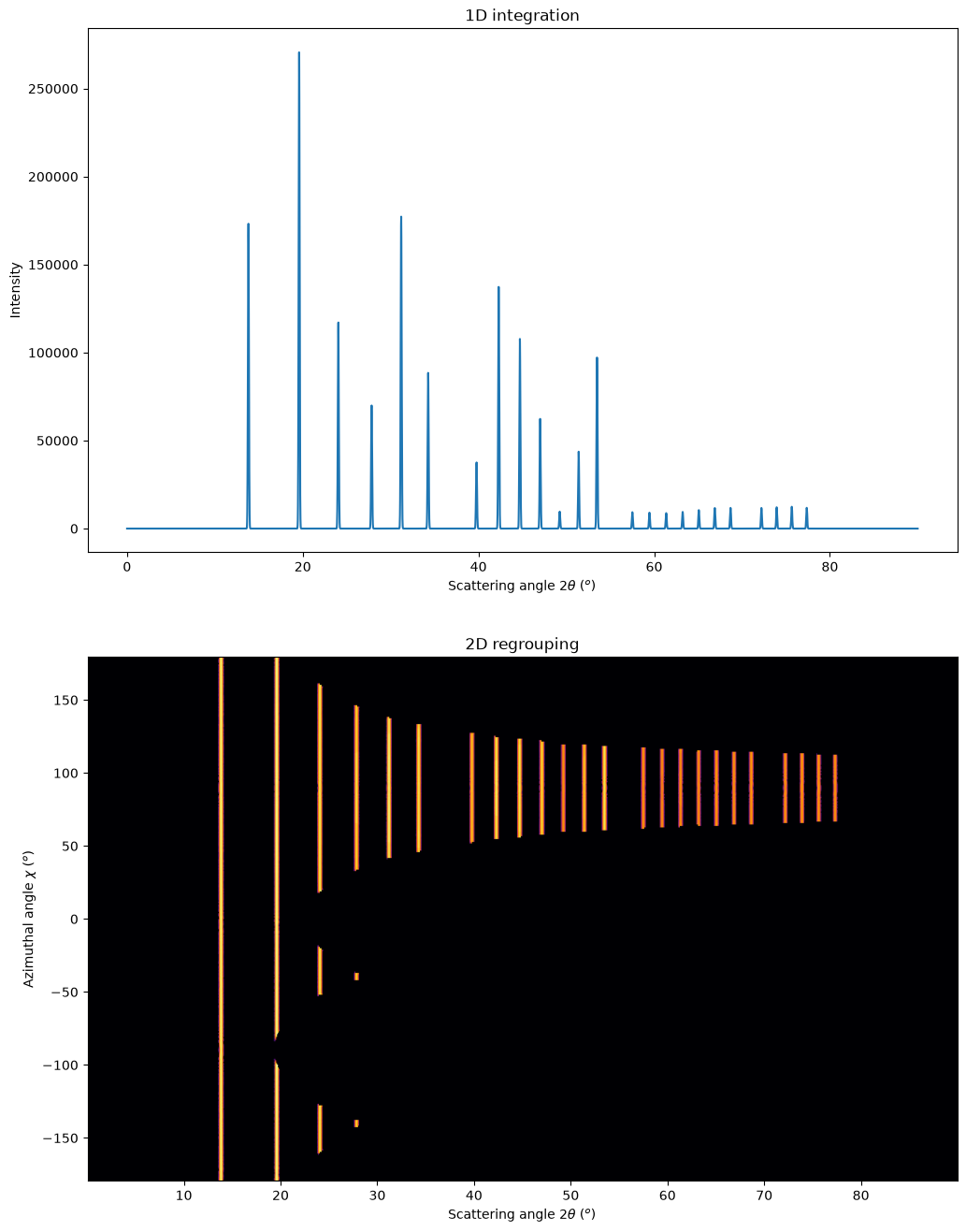
Creation of the MultiGeometry#
This time we will work in 2theta angle using degrees:
mg = MultiGeometry(ais, unit="2th_deg", radial_range=(0, 90))
print(mg)
fig, ax = subplots(2, 1, figsize=(12,16))
jupyter.plot1d(mg.integrate1d(imgs, 10000, method=method),
               ax=ax[0])
res2d = mg.integrate2d(imgs, 1000,360)
jupyter.plot2d(res2d, ax=ax[1]);
MultiGeometry integrator with 5 geometries on (0, 90) radial range ((2th_deg, chi_deg)) and None azimuthal range (deg)
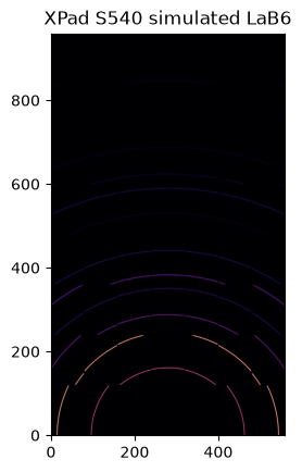
How to fill-up gaps in arrays of pixel detectors during 2D integration#
We will use an ImXpad detector which exhibits large gaps.
det = pyFAI.detectors.detector_factory("Xpad_flat")
p1, p2, p3 = det.calc_cartesian_positions()
print(p3)
poni1 = p1.mean()
poni2 = p2.mean()
print(poni1)
print(poni2)
None
0.074894994
0.03757
ai = pyFAI.load({"dist":0.1, "poni1":0, "poni2":poni2, "detector":det})
img = LaB6.fake_calibration_image(ai)
jupyter.display(img, label="XPad S540 simulated LaB6")
jupyter.plot2d(ai.integrate2d_ng(img, 500, 360, azimuth_range=(0,180), unit="2th_deg", dummy=-1, method=method2d),
               label="2D");
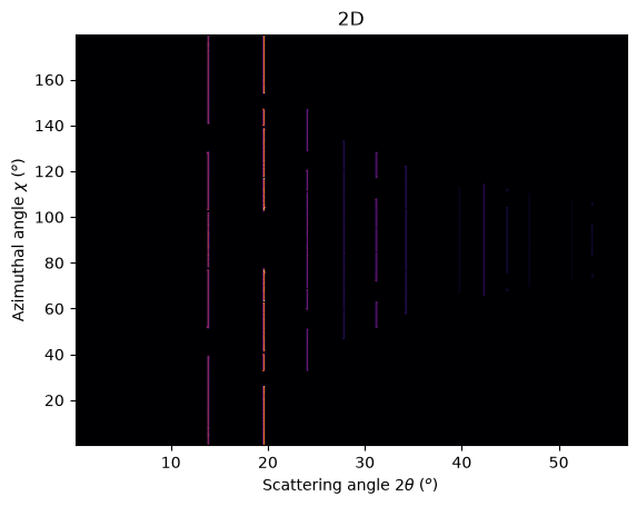
To observe textures, it is mandatory to fill the large empty space. This can be done by tilting the detector by a few degrees to higher 2theta angle (yaw 2x5deg) and turn the detector along the azimuthal angle (roll 2x5deg):
step = 5*numpy.pi/180
nb_geom = 3
ais = []
imgs = []
for i in range(nb_geom):
    for j in range(nb_geom):
        my_ai = copy.deepcopy(ai)
        my_ai.rot2 -= i*step
        my_ai.rot3 -= j*step
        my_img = LaB6.fake_calibration_image(my_ai)
        ais.append(my_ai)
        imgs.append(my_img)
mg = MultiGeometry(ais, unit="2th_deg", radial_range=(0, 60), azimuth_range=(0, 180), empty=-5)
print(mg)
res2d = mg.integrate2d(imgs, 1000, 360, method=method2d)
jupyter.plot2d(res2d, label="Filled");
MultiGeometry integrator with 9 geometries on (0, 60) radial range ((2th_deg, chi_deg)) and (0, 180) azimuthal range (deg)
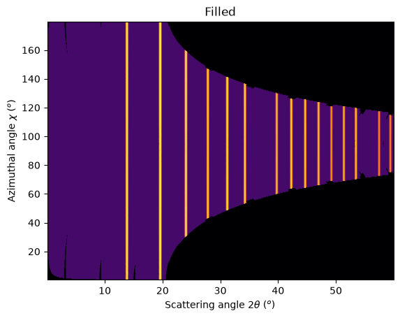
As one can see, the gaps have disappeared and the statistics are much better, except at the border where only one image contributes to the integrated image.
Conclusion#
The multi_geometry module of pyFAI makes powder diffraction experiments with small moving detectors much easier.
Some people prefer to stitch input images together prior to integration. There are plenty of good tools to do this: general ones like Photoshop or more specialized ones like AutoPano. More seriously, this can be done using the distortion module of a detector to re-sample the signal on a regular grid. However, one must store both the number of actual pixels contributing to a regular pixel and the total intensity contained within that regularised pixel. Without the former information, performing science with a rebinned image is as meaningful as using Photoshop.
print(f"Excution time: %.3f"%(time.perf_counter()-start_time))
Excution time: 40.157