Parallax effect

This tutorial demonstrates the parallax effect observed at large incidence angles with low-Z sensor materials.

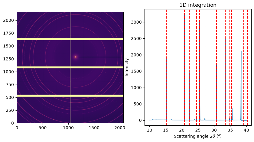
It uses one of the reference images available in the pyFAI test suite: a diffraction frame of corundum taken at ID13 with an Eiger detector and a beam of energy 13.45 keV.

Initialization

%matplotlib inline
import time
import copy
from matplotlib.pyplot import subplots
from scipy.sparse import csc_array
import fabio
import pyFAI
from pyFAI.gui import jupyter
from pyFAI.test.utilstest import UtilsTest
from pyFAI.calibrant import get_calibrant
import pyFAI.ext.parallax_raytracing

kwargs = {
    "npt": 2000,  # this is a lot of oversampling ... do not use with actual images.
    "method": (
        "no",
        "histogram",
        "cython",
    ),  # without pixel splitting, results are correct despite ugly images.
    "unit": "2th_deg",
    "radial_range": (10, 40),
    "dummy": 4e9,
    "delta_dummy": 1e9,
}

print(f"Using pyFAI version {pyFAI.version}")
start_time = time.perf_counter()

Using pyFAI version 2026.1.0-dev0

Display the image and the powder diffraction pattern

ai = pyFAI.load(UtilsTest.getimage("Eiger4M.poni"))
ai0 = copy.deepcopy(ai)  # this integrator does not know about parallax effect !
ai0

Detector Eiger 4M        PixelSize= 75µm, 75µm   BottomRight (3)
Wavelength= 0.921816 Å
SampleDetDist= 1.625582e-01 m   PONI= 9.632499e-02, 8.636842e-02 m      rot1=0.004596  rot2=0.000846  rot3=-0.000000 rad
DirectBeamDist= 162.560 mm      Center: x=1141.617, y=1286.167 pix      Tilt= 0.268° tiltPlanRotation= 169.572° λ= 0.922Å

alumine = get_calibrant("alpha_Al2O3")
alumine.wavelength = ai.wavelength

# Define sensor info to enable parallax:
ai.enable_parallax(True, sensor_material="Si", sensor_thickness=450e-6)
ai.detector.sensor = ai.parallax.sensor
ai

Detector Eiger 4M        PixelSize= 75µm, 75µm   BottomRight (3)         Thin sensor with µ=4108.472 1/m, thickness=0.00045m and efficiency=0.843
Wavelength= 0.921816 Å  Parallax: µ= 41.085 cm⁻¹
SampleDetDist= 1.625582e-01 m   PONI= 9.632499e-02, 8.636842e-02 m      rot1=0.004596  rot2=0.000846  rot3=-0.000000 rad
DirectBeamDist= 162.560 mm      Center: x=1141.617, y=1286.167 pix      Tilt= 0.268° tiltPlanRotation= 169.572° λ= 0.922Å

ai.energy

13.450000402192138

fig, ax = subplots(1, 2, figsize=(10, 5))
img_ref = fabio.open(UtilsTest.getimage("Eiger4M.edf")).data
jupyter.display(img_ref, ax=ax[0])
jupyter.plot1d(ai0.integrate1d(img_ref, **kwargs), ax=ax[1], calibrant=alumine);

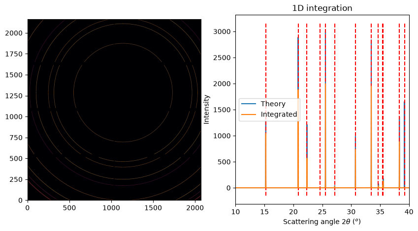
# prepare a synthetic dataset almost equivalent

ref_xrpd = alumine.fake_xrpdp(
    3000,
    (10, 40),
    resolution=1e-2,  # very fine resolution, finer than the pixel size
    unit="2th_deg",
    Imax=3e3,
)
img_ref = ai0.calcfrom1d(ref_xrpd.radial, ref_xrpd.intensity, mask=ai.detector.mask)
reintegrated = ai0.integrate1d(img_ref, **kwargs)

fig, ax = subplots(1, 2, figsize=(10, 5))
jupyter.display(img_ref, ax=ax[0])
jupyter.plot1d(ref_xrpd, ax=ax[1], calibrant=alumine, label="Theory")
ax[1].plot(*reintegrated, label="Integrated")
ax[1].set_xlim(10, 40)
ax[1].legend();

Calculate the bluring operator as a sparse matrix

rt = pyFAI.ext.parallax_raytracing.Raytracing(ai, buffer_size=32)

%%time
sparse = csc_array(
    rt.calc_csr(32),  # throw 32x32=1024 rays per pixel ... can take a while
    shape=(img_ref.size, img_ref.size),
)

CPU times: user 8min 51s, sys: 535 ms, total: 8min 51s
Wall time: 11.3 s

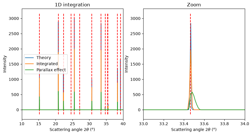
Apply parallax bluring on the image as sparse matrix multiplication:

img_par = sparse.dot(img_ref.ravel()).reshape(img_ref.shape)

res0 = ai0.integrate1d(img_ref, **kwargs)
res1 = ai0.integrate1d(img_par, **kwargs)

fig, ax = subplots(1, 2, figsize=(10, 5))
jupyter.plot1d(ref_xrpd, label="Theory", ax=ax[0], calibrant=alumine)
jupyter.plot1d(ref_xrpd, ax=ax[1], calibrant=alumine)
ax[0].plot(*res0, label="Integrated")
ax[1].plot(*res0, label="Integrated")
ax[0].plot(*res1, label="Parallax effect")
ax[1].plot(*res1, label="Parallax effect")
ax[0].set_xlim(10, 40)
ax[1].set_xlim(33, 34)
ax[1].set_title("Zoom")
ax[0].legend();

Correction of the parallax effect within the integrator

# Use the sensor material aware azimuthal integrator:
res2 = ai.integrate1d(img_par, **kwargs)

fig, ax = subplots(1, 2, figsize=(10, 5))
jupyter.plot1d(ref_xrpd, label="Theory", ax=ax[0], calibrant=alumine)
jupyter.plot1d(ref_xrpd, ax=ax[1], calibrant=alumine)
ax[0].plot(*res0, label="Integrated")
ax[1].plot(*res0, label="Integrated")
ax[0].plot(*res1, label="Parallax effect")
ax[1].plot(*res1, label="Parallax effect")

ax[0].plot(*res2, label="Parallax corrected")
ax[1].plot(*res2, label="Parallax corrected")

ax[0].set_xlim(10, 40)
ax[1].set_xlim(33.3, 33.6)

ax[1].set_title("Zoom")
ax[0].legend();

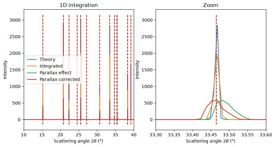
As shown, when the parallax correction is activated in the geometry/azimuthal integrator, the peak position (maximum) is shifted to the correct value. However, this correction does not deconvolve the peak shape (it does not remove the broadening introduced by parallax).

Conclusion

PyFAI provides tools to simulate the parallax effect using raytracing. The sparse matrix obtained can be used to blur a diffraction image and later to deconvolve it using iterative methods like MLEM. It is also able to take volumetric absorption effects into account to correct the peak position.

print(f"Runtime: {time.perf_counter() - start_time:.3f}s")

Runtime: 16.994s