Variance of SAXS data#
There has been a long discussion about the validity (or not) of pixel splitting regarding the propagation of errors #520 #882 #883. So we will develop a mathematical model for a SAXS experiment and validate it in the case of a SAXS approximation (i.e. no solid-angle correction, no polarisation effect, and of course small angled $\theta = sin(\theta) = tan(\theta)$)
System under study#
Let’s do a numerical experiment, simulating the following experiment:
Detector: 1024x1024 square pixels of 100µm each, assumed to be poissonian.
Geometry: The detector is placed at 1m from the sample, the beam center is in the corner of the detector
Intensity: the maximum signal on the detector is 10 000 photons per pixel, each pixel having a minimum count of a hundreed.
Wavelength: 1 Angstrom
During the first part of the studdy, the solid-angle correction will be discarded, same for polarisation corrections.
Since pixel splitting is disabled, many rebinning engines are available and will be benchmarked:
numpy: the slowest available in pyFAI
histogram: implemented in cython
nosplit_csr: using a look-up table
nosplit_csr_ocl_gpu: which offloads the calculation on the GPU.
We will check they all provide the same numerical result
Now we define some constants for the studdy. The dictionary kwarg contains the parameters used for azimuthal integration. This ensures the number of bins for the regrouping or correction like $\Omega$ and polarization are always the same.
%matplotlib inline
# use `widget` instead of `inline` for better user-exeperience. `inline` allows to store plots into notebooks.
import time
start_time = time.perf_counter()
import sys
print(sys.executable)
print(sys.version)
import os
os.environ["PYOPENCL_COMPILER_OUTPUT"] = "0"
/users/kieffer/.venv/py313/bin/python
3.13.1 | packaged by conda-forge | (main, Jan 13 2025, 09:53:10) [GCC 13.3.0]
pix = 100e-6
shape = (1024, 1024)
npt = 1000
nimg = 1000
wl = 1e-10
I0 = 1e4
kwargs = {"npt":npt,
         "correctSolidAngle":False,
         "polarization_factor":None,
         "safe":False}
import numpy, numexpr, numba
from scipy.stats import chi2 as chi2_dist
from matplotlib.pyplot import subplots
from matplotlib.colors import LogNorm
import logging
logging.basicConfig(level=logging.ERROR)
import pyFAI
print(f"pyFAI version: {pyFAI.version}")
from pyFAI.detectors import Detector
from pyFAI.method_registry import IntegrationMethod
from pyFAI.gui import jupyter
detector = Detector(pix, pix)
detector.shape = detector.max_shape = shape
print(detector)
pyFAI version: 2025.11.0-dev0
Detector Detector	 PixelSize= 100µm, 100µm	 BottomRight (3)
We define in ai_init the geometry, the detector and the wavelength.
ai_init = {"dist":1.0,
           "poni1":0.0,
           "poni2":0.0,
           "rot1":0.0,
           "rot2":0.0,
           "rot3":0.0,
           "detector":detector,
           "wavelength":wl}
ai = pyFAI.load(ai_init)
print(ai)

#Solid consideration:
Ω  = ai.solidAngleArray(detector.shape, absolute=True)

print(f"Solid angle: maxi= {Ω.max()} mini= {Ω.min()}, ratio= {Ω.min()/Ω.max()}")
Detector Detector	 PixelSize= 100µm, 100µm	 BottomRight (3)
Wavelength= 1.000000 Å
SampleDetDist= 1.000000e+00 m	PONI= 0.000000e+00, 0.000000e+00 m	rot1=0.000000  rot2=0.000000  rot3=0.000000 rad
DirectBeamDist= 1000.000 mm	Center: x=0.000, y=0.000 pix	Tilt= 0.000° tiltPlanRotation= 0.000° λ= 1.000Å
Solid angle: maxi= 9.999999925000007e-09 mini= 9.69376805173843e-09, ratio= 0.9693768124441684
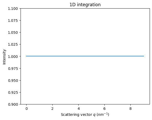
# Validation of the flatness of a flat image integrated
flat = numpy.ones(detector.shape)
res_flat = ai.integrate1d(flat, **kwargs)
crv = jupyter.plot1d(res_flat)
crv.axes.set_ylim(0.9,1.1);
#Equivalence of different rebinning engines ... looking for the fastest:
fastest = sys.maxsize
best = None
print(f"| {'Method':70s} | {'error':8s} | {'time(ms)':7s}|")
print("+"+"-"*72+"+"+"-"*10+"+"+"-"*9+"+")
for method in IntegrationMethod.select_method(dim=1):
    res_flat = ai.integrate1d(flat, method=method, **kwargs)
    #print(f"timeit for {method} max error: {abs(res_flat.intensity-1).max()}")
    m = str(method).replace(")","")[26:96]
    err = abs(res_flat.intensity-1).max()

    tm = %timeit -o -r1 -q ai.integrate1d(flat, method=method, **kwargs)
    tm_best = tm.best
    print(f"| {m:70s} | {err:6.2e} | {tm_best*1000:7.3f} |")
    if tm_best<fastest:
        fastest = tm_best
        best = method
print("+"+"-"*72+"+"+"-"*10+"+"+"-"*9+"+")
print(f"\nThe fastest method is {best} in {1000*fastest:.3f} ms/1Mpix frame")
| Method                                                                 | error    | time(ms)|
+------------------------------------------------------------------------+----------+---------+
| no split, histogram, python                                            | 0.00e+00 |  31.282 |
| no split, histogram, cython                                            | 0.00e+00 |  10.548 |
| bbox split, histogram, cython                                          | 0.00e+00 |  26.862 |
| full split, histogram, cython                                          | 0.00e+00 | 180.475 |
| no split, CSR, cython                                                  | 0.00e+00 |  20.511 |
| bbox split, CSR, cython                                                | 0.00e+00 |  20.392 |
| no split, CSR, python                                                  | 0.00e+00 |  10.554 |
| bbox split, CSR, python                                                | 0.00e+00 |  11.910 |
| no split, CSC, cython                                                  | 0.00e+00 |   8.844 |
| bbox split, CSC, cython                                                | 0.00e+00 |  10.568 |
| no split, CSC, python                                                  | 0.00e+00 |  10.835 |
| bbox split, CSC, python                                                | 0.00e+00 |  14.001 |
| bbox split, LUT, cython                                                | 0.00e+00 |  21.563 |
| no split, LUT, cython                                                  | 0.00e+00 |  20.425 |
| full split, LUT, cython                                                | 0.00e+00 |  20.233 |
| full split, CSR, cython                                                | 0.00e+00 |  21.594 |
| full split, CSR, python                                                | 0.00e+00 |  11.618 |
| full split, CSC, cython                                                | 0.00e+00 |  10.400 |
| full split, CSC, python                                                | 0.00e+00 |  13.794 |
/users/kieffer/.venv/py313/lib/python3.13/site-packages/pyopencl/__init__.py:519: CompilerWarning: Non-empty compiler output encountered. Set the environment variable PYOPENCL_COMPILER_OUTPUT=1 to see more.
  lambda: self._prg.build(options_bytes, devices),
| no split, histogram, OpenCL, NVIDIA CUDA / NVIDIA RTX A5000            | 1.19e-07 |   6.241 |
| no split, histogram, OpenCL, NVIDIA CUDA / Quadro P2200                | 1.19e-07 |   5.396 |
1 error generated.
| no split, histogram, OpenCL, Portable Computing Language / cpu-haswell | 0.00e+00 | 13.949 |
/users/kieffer/.venv/py313/lib/python3.13/site-packages/pyopencl/cache.py:420: CompilerWarning: Non-empty compiler output encountered. Set the environment variable PYOPENCL_COMPILER_OUTPUT=1 to see more.
  prg.build(options_bytes, [devices[i] for i in to_be_built_indices])
| no split, histogram, OpenCL, Intel(R OpenCL / AMD Ryzen Threadripper P | 0.00e+00 |  11.940 |
| bbox split, CSR, OpenCL, NVIDIA CUDA / NVIDIA RTX A5000                | 1.19e-07 |   0.959 |
| no split, CSR, OpenCL, NVIDIA CUDA / NVIDIA RTX A5000                  | 1.19e-07 |   0.902 |
| bbox split, CSR, OpenCL, NVIDIA CUDA / Quadro P2200                    | 1.19e-07 |   1.334 |
| no split, CSR, OpenCL, NVIDIA CUDA / Quadro P2200                      | 1.19e-07 |   1.218 |
| bbox split, CSR, OpenCL, Portable Computing Language / cpu-haswell-AMD | 0.00e+00 |   4.739 |
| no split, CSR, OpenCL, Portable Computing Language / cpu-haswell-AMD R | 0.00e+00 |   4.269 |
| bbox split, CSR, OpenCL, Intel(R OpenCL / AMD Ryzen Threadripper PRO 3 | 0.00e+00 |   3.933 |
/users/kieffer/.venv/py313/lib/python3.13/site-packages/pyopencl/cache.py:496: CompilerWarning: Non-empty compiler output encountered. Set the environment variable PYOPENCL_COMPILER_OUTPUT=1 to see more.
  _create_built_program_from_source_cached(
/users/kieffer/.venv/py313/lib/python3.13/site-packages/pyopencl/cache.py:500: CompilerWarning: Non-empty compiler output encountered. Set the environment variable PYOPENCL_COMPILER_OUTPUT=1 to see more.
  prg.build(options_bytes, devices)
| no split, CSR, OpenCL, Intel(R OpenCL / AMD Ryzen Threadripper PRO 397 | 0.00e+00 |   3.348 |
| full split, CSR, OpenCL, NVIDIA CUDA / NVIDIA RTX A5000                | 1.19e-07 |   1.065 |
| full split, CSR, OpenCL, NVIDIA CUDA / Quadro P2200                    | 1.19e-07 |   1.374 |
| full split, CSR, OpenCL, Portable Computing Language / cpu-haswell-AMD | 0.00e+00 |   4.690 |
| full split, CSR, OpenCL, Intel(R OpenCL / AMD Ryzen Threadripper PRO 3 | 0.00e+00 |   4.299 |
| bbox split, LUT, OpenCL, NVIDIA CUDA / NVIDIA RTX A5000                | 1.19e-07 |   3.317 |
| no split, LUT, OpenCL, NVIDIA CUDA / NVIDIA RTX A5000                  | 1.19e-07 |   2.576 |
| bbox split, LUT, OpenCL, NVIDIA CUDA / Quadro P2200                    | 1.19e-07 |   3.295 |
| no split, LUT, OpenCL, NVIDIA CUDA / Quadro P2200                      | 1.19e-07 |   2.781 |
| bbox split, LUT, OpenCL, Portable Computing Language / cpu-haswell-AMD | 0.00e+00 |   5.840 |
| no split, LUT, OpenCL, Portable Computing Language / cpu-haswell-AMD R | 0.00e+00 |   4.741 |
| bbox split, LUT, OpenCL, Intel(R OpenCL / AMD Ryzen Threadripper PRO 3 | 0.00e+00 |   4.900 |
| no split, LUT, OpenCL, Intel(R OpenCL / AMD Ryzen Threadripper PRO 397 | 0.00e+00 |   5.604 |
| full split, LUT, OpenCL, NVIDIA CUDA / NVIDIA RTX A5000                | 1.19e-07 |   3.289 |
| full split, LUT, OpenCL, NVIDIA CUDA / Quadro P2200                    | 1.19e-07 |   3.257 |
| full split, LUT, OpenCL, Portable Computing Language / cpu-haswell-AMD | 0.00e+00 |   5.386 |
| full split, LUT, OpenCL, Intel(R OpenCL / AMD Ryzen Threadripper PRO 3 | 0.00e+00 |   6.331 |
+------------------------------------------------------------------------+----------+---------+

The fastest method is IntegrationMethod(1d int, no split, CSR, OpenCL, NVIDIA CUDA / NVIDIA RTX A5000) in 0.902 ms/1Mpix frame
# so we chose the fastest method without pixel splitting ...other methods may be faster
kwargs["method"] = IntegrationMethod.select_method(dim=1,
                                                  split="no",
                                                  algo="csr",
                                                  impl="opencl",
                                                  target_type="gpu")[0]
print(kwargs["method"])
IntegrationMethod(1d int, no split, CSR, OpenCL, NVIDIA CUDA / NVIDIA RTX A5000)
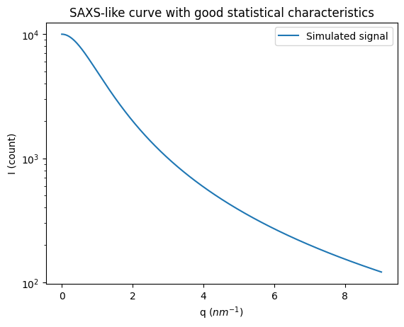
# Generation of a "SAXS-like" curve with the shape of a lorentzian curve

q = numpy.linspace(0, res_flat.radial.max(), npt)
I = I0/(1+q**2)
fig, ax = subplots()
ax.semilogy(q, I, label="Simulated signal")
ax.set_xlabel("q ($nm^{-1}$)")
ax.set_ylabel("I (count)")
ax.set_title("SAXS-like curve with good statistical characteristics")
ax.legend();
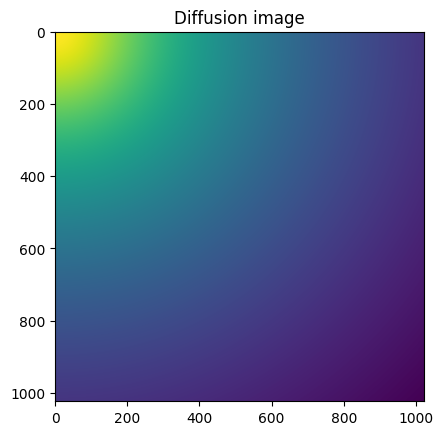
#Reconstruction of diffusion image:

img_theo = ai.calcfrom1d(q, I, dim1_unit="q_nm^-1",
                         correctSolidAngle=False,
                         polarization_factor=None)
fig, ax = subplots()
ax.imshow(img_theo, norm=LogNorm())
ax.set_title("Diffusion image");
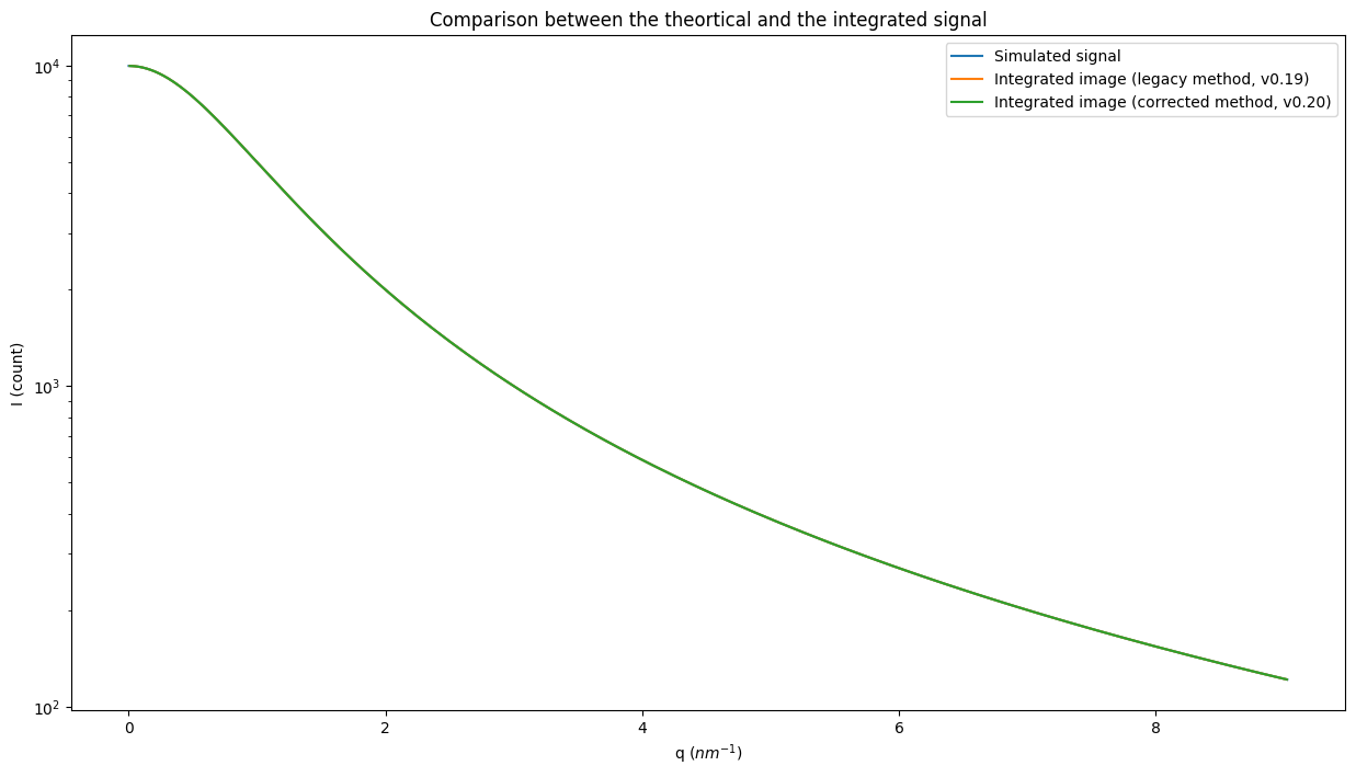
fig, ax = subplots(figsize=(15,8))
ax.semilogy(q, I, label="Simulated signal")
ax.set_xlabel("q ($nm^{-1}$)")
ax.set_ylabel("I (count)")
res_ng = ai.integrate1d_ng(img_theo, **kwargs)
res_legacy = ai.integrate1d_legacy(img_theo, **kwargs)
ax.plot(*res_legacy, label="Integrated image (legacy method, v0.19)")
ax.plot(*res_ng, label="Integrated image (corrected method, v0.20)")
ax.set_title("Comparison between the theortical and the integrated signal")
#Display the error: commented as it makes the graph less readable
#I_bins = I0/(1+res.radial**2)
#ax.plot(res.radial, abs(res.intensity-I_bins), label="error")
ax.legend();
Construction of a synthetic dataset#
We construct now a synthetic dataset of thousand images of this reference image with a statistical distribution which is common for photon-counting detectors (like Pilatus or Eiger): The Poisson distribution. The signal is between 100 and 10000, so every pixel should see photons and there is should be no “rare-events” bias (which sometimes occures in SAXS).
Poisson distribution:#
The Poisson distribution has the peculiarity of having its variance equal to the signal, hence the standard deviation equals to the square root of the signal.
Nota: the generation of the images is slow and takes about 1Gbyte of memory !
%%time

if "dataset" not in dir():
    dataset = numpy.random.poisson(img_theo, (nimg,) + img_theo.shape)
# else avoid wasting time
print(dataset.nbytes/(1<<20), "MBytes", dataset.shape)
8000.0 MBytes (1000, 1024, 1024)
CPU times: user 56.7 s, sys: 1.33 s, total: 58 s
Wall time: 58 s
Validation of the Poisson distribution.#
We have now thousand images of one magapixel. It is interesting to validate if the distribution actually follows the Poisson distribution. For this we will check if the signal and its variance follow a $\chi^2$ distribution.
For every pair of images I and J we calculate the numerical value of $\chi ^2$:
$$ \chi^2 = \frac{1}{nbpixel-1}\sum_{pix}\frac{(I_{pix} - J_{pix})^2}{\sigma(I_{pix})^2 + \sigma(J_{pix})^2)} $$
The distibution is obtained by calculating the histogram of $\chi^2$ values for every pair of images, here almost half a milion.
The calculation of the $\chi^2$ value is likely to be critical in time, so we will shortly investigate 3 implementation: numpy (fail-safe but not that fast), numexp and numba Do not worry if any of the two later method fail: they are faster but provide the same numerical result as numpy.
print("Number of paires of images: ", nimg*(nimg-1)//2)
Number of paires of images: 499500
#Numpy implementation of Chi^2 measurement for a pair of images. Fail-safe implementation

def chi2_images_np(I, J):
    """Calculate the Chi2 value for a pair of images with poissonnian noise
    Numpy implementation"""
    return ((I-J)**2/(I+J)).sum()/(I.size - 1)

img0 = dataset[0]
img1 = dataset[1]
print("𝜒² value calculated from numpy on the first pair of images:", chi2_images_np(img0, img1))
%timeit chi2_images_np(img0, img1)
𝜒² value calculated from numpy on the first pair of images: 1.000554455909926
5.88 ms ± 15.9 μs per loop (mean ± std. dev. of 7 runs, 100 loops each)
#Numexp implementation of Chi^2 measurement for a pair of images.
import numexpr
from numexpr import NumExpr
expr = NumExpr("((I-J)**2/(I+J))", signature=[("I", numpy.float64),("J", numpy.float64)])

def chi2_images_ne(I, J):
    """Calculate the Chi2 value for a pair of images with poissonnian noise
    NumExpr implementation"""
    return expr(I, J).sum()/(I.size-1)

img0 = dataset[0]
img1 = dataset[1]
print("𝜒² value calculated from numexpr on the first pair of images:",chi2_images_ne(img0, img1))
for i in range(6):
    j = 1<<i
    numexpr.set_num_threads(j)
    print(f"Timing when using {j} threads: ")
    %timeit -r 3 chi2_images_ne(img0, img1)

#May fail if numexpr is not installed, but gives the same numerical value, just faster
𝜒² value calculated from numexpr on the first pair of images: 1.000554455909926
Timing when using 1 threads:
4.54 ms ± 19.7 μs per loop (mean ± std. dev. of 3 runs, 100 loops each)
Timing when using 2 threads:
3.62 ms ± 755 μs per loop (mean ± std. dev. of 3 runs, 100 loops each)
Timing when using 4 threads:
4.83 ms ± 262 μs per loop (mean ± std. dev. of 3 runs, 100 loops each)
Timing when using 8 threads:
3.42 ms ± 180 μs per loop (mean ± std. dev. of 3 runs, 100 loops each)
Timing when using 16 threads:
2.48 ms ± 293 μs per loop (mean ± std. dev. of 3 runs, 100 loops each)
Timing when using 32 threads:
2.4 ms ± 220 μs per loop (mean ± std. dev. of 3 runs, 100 loops each)
#Numba implementation of Chi^2 measurement for a pair of images.
from numba import jit, njit, prange

@njit(parallel=True)
def chi2_images_nu(img1, img2):
    """Calculate the Chi2 value for a pair of images with poissonnian noise
    Numba implementation"""
    I = img1.ravel()
    J = img2.ravel()
    l = len(I)
    #assert len(J) == l
    #version optimized for JIT
    s = 0.0
    for i in prange(len(I)):
        a = float(I[i])
        b = float(J[i])
        s+= (a-b)**2/(a+b)
    return s/(l-1)

img0 = dataset[0]
img1 = dataset[1]
print("𝜒² value calculated from numba on the first pair of images:", chi2_images_nu(img0, img1))
%timeit chi2_images_nu(img0, img1)

#May fail if numba is not installed.
# The numerical value, may differ due to reduction algorithm used, should be the fastest.
𝜒² value calculated from numba on the first pair of images: 1.0005544559099273
329 μs ± 27.2 μs per loop (mean ± std. dev. of 7 runs, 1,000 loops each)
# Select the prefered algorithm for calculating the numerical value of chi^2 for a pair of images.
#chi2_images = chi2_images_ne
#numexpr.set_num_threads(16)
chi2_images = chi2_images_nu
%%time

#Calculate the numerical value for chi2 for every pair of images. This takes a while

c2i = []
for i in range(nimg):
    img1 = dataset[i]
    for img2 in dataset[:i]:
        c2i.append(chi2_images(img1, img2))
c2i = numpy.array(c2i)
CPU times: user 1h 41min 12s, sys: 41min 9s, total: 2h 22min 21s
Wall time: 4min 12s
fig, ax = subplots()
h,b,_ = ax.hist(c2i, 100, label="measured distibution")
ax.plot()
size = numpy.prod(shape)
y_sim = chi2_dist.pdf(b*(size-1), size)
y_sim *= h.sum()/y_sim.sum()
ax.plot(b, y_sim, label=r"$\chi^2$ distribution")
ax.set_title("Is the set of images Poissonian?")
ax.legend();
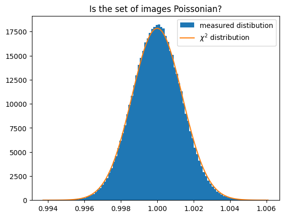
This validates the fact that our set of image is actually a Poissonian distribution around the target image displayed in figure 3.
Integration of images in the SAXS appoximation:#
We can now integrate all images and check wheather all pairs of curves (with their associated error) fit or not the $\chi^2$ distribution.
It is important to remind that we stay in SAXS approximation, i.e. no solid angle correction or other position-dependent normalization. The pixel splitting is also disabled. So the azimuthal integration is simply:
$$ I_{bin} = \frac{1}{count(pix\in bin)} \sum_{pix \in bin} I_{pix} $$
The number of bins in the curve being much smaller than the number of pixel in the input image, this calculation is less time-critical. So we simply define the same kind of $\chi^2$ function using numpy.
def chi2_curves(res1, res2):
    """Calculate the Chi2 value for a pair of integrated data"""
    I = res1.intensity
    J = res2.intensity
    l = len(I)
    assert len(J) == l
    sigma_I = res1.sigma
    sigma_J = res2.sigma
    return ((I-J)**2/(sigma_I**2+sigma_J**2)).sum()/(l-1)
%%time
#Perform the azimuthal integration of every single image

integrated = [ai.integrate1d_legacy(data, variance=data, **kwargs)
             for data in dataset]
CPU times: user 2.23 s, sys: 0 ns, total: 2.23 s
Wall time: 2.24 s
#Check if chi^2 calculation is time-critical:
%timeit chi2_curves(integrated[0], integrated[1])
6.46 μs ± 14.2 ns per loop (mean ± std. dev. of 7 runs, 100,000 loops each)
%%time
c2 = []
for i in range(nimg):
    res1 = integrated[i]
    for res2 in integrated[:i]:
        c2.append(chi2_curves(res1, res2))
c2 = numpy.array(c2)
CPU times: user 3.33 s, sys: 0 ns, total: 3.33 s
Wall time: 3.33 s
fig, ax = subplots()
h,b,_ = ax.hist(c2, 100, label="Measured distibution")
y_sim = chi2_dist.pdf(b*(npt-1), npt)
y_sim *= h.sum()/y_sim.sum()
ax.plot(b, y_sim, label=r"Chi^2 distribution")
ax.set_title("Integrated curves in SAXS approximation")
ax.legend();
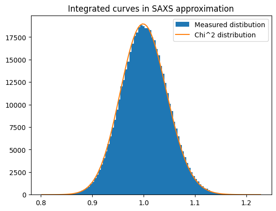
low_lim, up_lim = chi2_dist.ppf([0.005, 0.995], nimg) / (nimg - 1)
print(low_lim, up_lim)
print("Expected outliers: ", nimg*(nimg-1)*0.005/2, "got",
(c2<low_lim).sum(),"below and ",(c2>up_lim).sum(), "above")
0.889452976157626 1.1200681344576493
Expected outliers:  2497.5 got 2385 below and  2957 above
Integration of images with solid angle correction/polarization correction#
PyFAI applies by default solid-angle correction which is needed for powder diffraction. On synchrotron sources, the beam is highly polarized and one would like to correct for this effect as well. How does it influence the error propagation ?
If we enable the solid angle normalisation (noted $\Omega$) and the polarisation correction (noted $P$), this leads us to:
$$ I_{bin} = \frac{1}{count(pix\in bin)} \sum_{pix \in bin} \frac{I_{pix}}{\Omega_{pix} P_{pix}} $$
Flatfield correction and any other normalization like pixel efficiency related to sensor thickness should be accounted in the same way.
Nota: The pixel splitting remains disabled.
kwargs = {"npt":npt,
"correctSolidAngle": True,
"polarization_factor": 0.9,
"error_model": "poisson",
"safe":False}
kwargs["method"] = IntegrationMethod.select_method(dim=1,
split="no",
algo="csr",
impl="opencl",
target_type="gpu")[-1]
print(kwargs["method"])
# Since we use "safe"=False, we need to reset the integrator manually:
ai.reset()
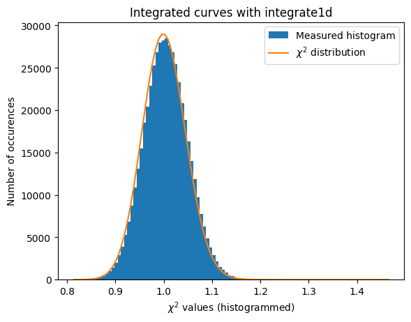
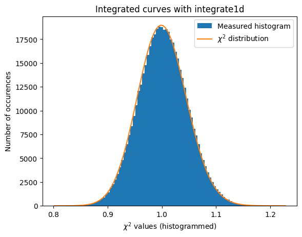
def plot_distribution(ai, kwargs, nbins=100, integrate=None, ax=None):
ai.reset()
results = []
c2 = []
if integrate is None:
integrate = ai._integrate1d_legacy
for i in range(nimg):
data = dataset[i, :, :]
r = integrate(data, **kwargs)
results.append(r)
for j in results[:i]:
c2.append(chi2_curves(r, j))
c2 = numpy.array(c2)
if ax is None:
fig, ax = subplots()
h,b,_ = ax.hist(c2, nbins, label="Measured histogram")
y_sim = chi2_dist.pdf(b*(npt-1), npt)
y_sim *= h.sum()/y_sim.sum()
ax.plot(b, y_sim, label=r"$\chi^{2}$ distribution")
ax.set_title(f"Integrated curves with {integrate.__name__}")
ax.set_xlabel("$\chi^{2}$ values (histogrammed)")
ax.set_ylabel("Number of occurences")
ax.legend()
return ax
a=plot_distribution(ai, kwargs)
IntegrationMethod(1d int, no split, CSR, OpenCL, NVIDIA CUDA / Quadro P2200)

The normalisation of the raw signal distorts the distribution of error, even at a level of a few percent correction ! (Thanks Daniel Franke for the demonstration)
Introducing the new generation of azimuthal integrator … in production since 0.20#
As any normalization introduces some distortion into the error propagation, the error propagation should properly account for this. Alessandro Mirone suggested to treat normalization within azimuthal integration like this :
$$ I_{bin} = \frac{\sum_{pix \in bin} I_{pix}}{\sum_{pix \in bin} \Omega_{pix}P_{pix}} $$
This is under investigation since begining 2017 https://github.com/silx-kit/pyFAI/issues/520 and is now available in production.
Nota: This is a major issue as almost any commercial detector comes with flatfield correction already applied on raw images; making impossible to properly propagate the error (I am especially thinking at photon counting detectors manufactured by Dectris!). The detector should then provide the actual raw-signal and the flatfield normalization to allow proper signal and error propagation.
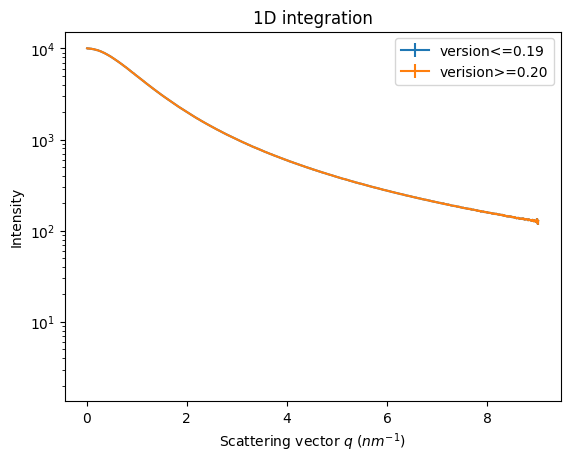
Here is a comparison between the legacy integrators and the new generation ones:
#The new implementation provides almost the same result as the former one:
ai.reset()
fig, ax = subplots()
data = dataset[0]
ax.set_yscale("log")
jupyter.plot1d(ai.integrate1d_legacy(data, **kwargs), ax=ax, label="version<=0.19")
jupyter.plot1d(ai.integrate1d_ng(data, **kwargs), ax=ax, label="verision>=0.20")
ax.legend();
# If you zoom in enough, you will see the difference !
#Validation of the error propagation without pixel splitting but with normalization:
a=plot_distribution(ai, kwargs, integrate = ai.integrate1d_ng)

#Validation of the error propagation without pixel splitting with azimuthal error assessement
kw_azim = kwargs.copy()
kw_azim["error_model"] = "azimuthal"
kw_azim["correctSolidAngle"] = False
kw_azim["polarization_factor"] = None


a=plot_distribution(ai, kw_azim, integrate = ai.integrate1d_ng)
#what if we use weights (solid-angle, polarization, ...) together with azimuthal error assessement ?
#Validation of the error propagation without pixel splitting with azimuthal error assessement
kw_azim = kwargs.copy()
kw_azim["error_model"] = "azimuthal"
kw_azim["correctSolidAngle"] = True
kw_azim["polarization_factor"] = 0.95


a=plot_distribution(ai, kw_azim, integrate = ai.integrate1d_ng)

The azimuthal error model is not correct yet … work needs to go on in that direction.
Azimuthal integration with pixel splitting#
Pixels splitting is implemented in pyFAI in calculating the fraction of area every pixel spends in any bin. This is noted $c^{pix}{bin}$. The calculation of those coeficient is done with some simple geometry but it is rather tedious, this is why two implementation exists: a simple one which assues pixels boundary are paralle to the radial and azimuthal axes called bbox for bounding box and a more precise one calculating the intersection of polygons (called full. The calculation of those coefficient is what lasts during the initialization of the integrator as this piece of code is not (yet) parallelized. The total number of (complete) pixel in a bin is then simply the sum of all those coeficients: $\sum{pix \in bin} c^{pix}_{bin}$.
The azimuthal integration used to be implemented as (pyFAI <=0.15):
$$ I_{bin} = \frac{ \sum_{pix \in bin} c^{pix}{bin} \frac{I{pix}}{\Omega_{pix} P_{pix}}}{\sum_{pix \in bin}c^{pix}_{bin}} $$
With the associated error propagation (with the error!):
$$ \sigma_{bin} = \frac{\sqrt{\sum_{pix \in bin} c^{pix}{bin} \sigma^2{pix}}}{\sum_{pix \in bin}c^{pix}_{bin}} $$
The new generation of integrator in production since version 0.20 (in 1D at least) are implemented like this:
$$ I_{bin} = \frac{\sum_{pix \in bin} c^{pix}{bin}I{pix}}{\sum_{pix \in bin} c^{pix}{bin}\Omega{pix}P_{pix}} $$
the associated variance propagation should look like this:
$$ \sigma_{bin} = \frac{\sqrt{\sum_{pix \in bin} (c^{pix}{bin})^2 \sigma^2{pix}}} {\sum_{pix \in bin}c^{pix}{bin}\Omega{pix}P_{pix}} $$
Since we have now tools to validate the error propagation for every single rebinning engine. Let’s see if pixel splitting induces some error, with coarse or fine pixel splitting:
#With coarse pixel-splitting, new integrator:
kwargs["method"] = IntegrationMethod.select_method(dim=1,
                                                   split="bbox",
                                                   algo="csr",
                                                   impl="opencl",
                                                   target_type="gpu")[-1]
print(kwargs["method"])
a = plot_distribution(ai, kwargs, integrate = ai.integrate1d_ng)
IntegrationMethod(1d int, bbox split, CSR, OpenCL, NVIDIA CUDA / Quadro P2200)

#With fine pixel-splitting, new integrator:
# so we chose the nosplit_csr_ocl_gpu, other methods may be faster depending on the computer
kwargs["method"] = IntegrationMethod.select_method(dim=1,
                                                   split="full",
                                                   algo="csr",
                                                   impl="opencl",
                                                   target_type="gpu")[-1]
print(kwargs["method"])
a = plot_distribution(ai, kwargs, integrate = ai.integrate1d_ng)
IntegrationMethod(1d int, full split, CSR, OpenCL, NVIDIA CUDA / Quadro P2200)

With those modification available, we are now able to estimate the error propagated from one curve and compare it with the “usual” result from pyFAI:
The integrated curves are now following the $\chi^2$ distribution, which means that the errors provided are in accordance with the data.
# Python histogramming without pixels splitting.

kwargs = {"npt":npt,
          "method": ("no", "histogram", "python"),
          "correctSolidAngle": True,
          "polarization_factor": 0.9,
          "safe": False,
          "error_model": "poisson"}
a = plot_distribution(ai, kwargs, integrate=ai._integrate1d_ng)
# Cython histogramming without pixels splitting.

kwargs = {"npt":npt,
          "method": ("no", "histogram", "cython"),
          "correctSolidAngle": True,
          "polarization_factor": 0.9,
          "safe": False,
          "error_model": "poisson"}
a = plot_distribution(ai, kwargs, integrate=ai._integrate1d_ng)

# OpenCL histogramming without pixels splitting.

kwargs = {"npt":npt,
         "method": ("no", "histogram", "opencl"),
         "correctSolidAngle": True,
         "polarization_factor": 0.9,
         "safe": False,
         "error_model": "poisson"}
a = plot_distribution(ai, kwargs, integrate=ai._integrate1d_ng)

Conclusion#
PyFAI’s historical version (version <=0.16) has been providing proper error propagation ONLY in the case where any normalization (solid angle, flatfield, polarization, …) and pixel splitting was DISABLED. This notebook demonstrates the correctness of the new integrator. Moreover the fact the normalization is performed as part of the integration is a major issue as almost any commercial detector comes with flatfield correction already applied.
print(f"Total execution time: {time.perf_counter()-start_time:.3f} s")
Total execution time: 559.558 s