Re-calibration of a diffraction image with Jupyter#
Jupyter notebooks (and jupyterlab) are standard tools to perfrom data analysis. While there are plenty of tutorial on the usage of pyFAI for azimuthal integration, few of then address the need for calculating the geometry of the experimental setup, also because the tool is not yet completely ready…
In this example we will perform the precise calibration of an image which setup is roughly known.
%matplotlib inline
# use `widget` for better user user experience; `inline` is for documentation generation

import time
from matplotlib.pyplot import subplots
from pyFAI.gui import jupyter
import pyFAI
import fabio
from pyFAI.test.utilstest import UtilsTest
from pyFAI.calibrant import CALIBRANT_FACTORY
from pyFAI.goniometer import SingleGeometry
print(f"Using pyFAI version: {pyFAI.version}")
start_time = time.perf_counter()
Using pyFAI version: 2025.11.0-dev0
# In this example, we will re-use one of the image used int the test-suite
filename = UtilsTest.getimage("Pilatus1M.edf")
frame = fabio.open(filename).data
# and now display the image
ax = jupyter.display(frame)
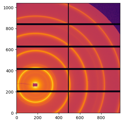
# This allow to measure approximatively the position of the beam center ...
x = 200 # x-coordinate of the beam-center in pixels
y = 300 # y-coordinate of the beam-center in pixels
d = 1600 # This is the distance in mm (unit used by Fit2d)
wl = 1e-10 # The wavelength is 1 Å
# Definition of the detector and of the calibrant:
pilatus = pyFAI.detector_factory("Pilatus1M")
behenate = CALIBRANT_FACTORY("AgBh")
behenate.wavelength = wl
behenate
AgBh Calibrant with 49 reflections at wavelength 1e-10
# Set the guessed geometry
initial = pyFAI.geometry.Geometry(detector=pilatus, wavelength=wl)
initial.setFit2D(d,x,y)
initial
Detector Pilatus 1M	 PixelSize= 172µm, 172µm	 BottomRight (3)
Wavelength= 1.000000 Å
SampleDetDist= 1.600000e+00 m	PONI= 5.160000e-02, 3.440000e-02 m	rot1=0.000000  rot2=0.000000  rot3=0.000000 rad
DirectBeamDist= 1600.000 mm	Center: x=200.000, y=300.000 pix	Tilt= 0.000° tiltPlanRotation= 0.000° λ= 1.000Å
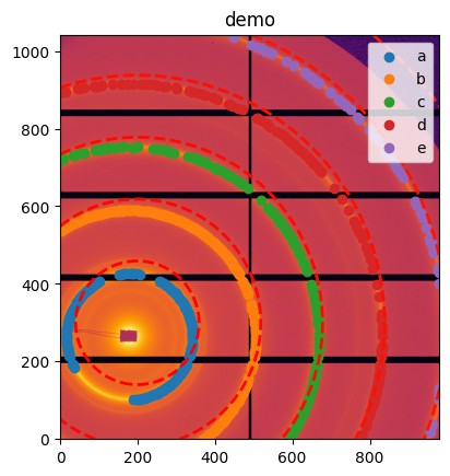
# The SingleGeometry object (from goniometer) allows to extract automatically ring and calibrate
sg = SingleGeometry("demo", frame, calibrant=behenate, detector=pilatus, geometry=initial)
sg.extract_cp(max_rings=5)
ControlPoints instance containing 5 group of point:
AgBh Calibrant with 49 reflections at wavelength 1e-10
Containing 5 groups of points:
# a ring 0: 177 points
# b ring 1: 206 points
# c ring 2: 151 points
# d ring 3: 133 points
# e ring 4: 67 points
#Control point and rings do not overlap well initially (this was a guessed geometry)
ax = jupyter.display(sg=sg)
# Refine the geometry ... here in SAXS geometry, the rotation is fixed in orthogonal setup
sg.geometry_refinement.refine2(fix=["rot1", "rot2", "rot3", "wavelength"])
sg.get_ai()
Detector Pilatus 1M	 PixelSize= 172µm, 172µm	 BottomRight (3)
Wavelength= 1.000000 Å
SampleDetDist= 1.634776e+00 m	PONI= 4.543538e-02, 3.094137e-02 m	rot1=0.000000  rot2=0.000000  rot3=0.000000 rad
DirectBeamDist= 1634.776 mm	Center: x=179.892, y=264.159 pix	Tilt= 0.000° tiltPlanRotation= 0.000° λ= 1.000Å
ax = jupyter.display(sg=sg)

#Save the geometry obtained
sg.geometry_refinement.save("geometry.poni")
with open("geometry.poni") as f:
    print(f.read())
# Nota: C-Order, 1 refers to the Y axis, 2 to the X axis
# Calibration done at Tue Jan 10 13:20:21 2023
poni_version: 2
Detector: Pilatus1M
Detector_config: {}
Distance: 1.63465025483624
Poni1: 0.04543748793640355
Poni2: 0.030944866193985884
Rot1: 0.0
Rot2: 0.0
Rot3: 0
Wavelength: 1e-10
# Nota: C-Order, 1 refers to the Y axis, 2 to the X axis
# Calibration done at Tue Oct 10 17:17:00 2023
poni_version: 2
Detector: Pilatus1M
Detector_config: {}
Distance: 1.634722545051207
Poni1: 0.045434783654226624
Poni2: 0.030941659740724374
Rot1: 0.0
Rot2: 0.0
Rot3: 0
Wavelength: 1e-10
# Nota: C-Order, 1 refers to the Y axis, 2 to the X axis
# Calibration done on Sun Nov 16 15:01:20 2025
poni_version: 2.1
Detector: Pilatus1M
Detector_config: {"pixel1": 0.000172, "pixel2": 0.000172, "orientation": 3}
Distance: 1.6347759568952076
Poni1: 0.0454353809768665
Poni2: 0.030941365874399936
Rot1: 0.0
Rot2: 0.0
Rot3: 0
Wavelength: 1e-10
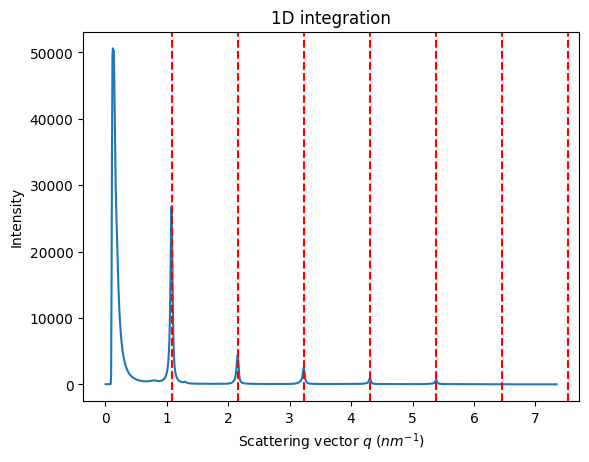
#Use the geometry to perform an azimuthal integration
ai = sg.get_ai()
res = ai.integrate1d(frame, 1000)
ax = jupyter.plot1d(res,calibrant=behenate)
Conclusion#
PyFAI still lacks some good integration into the Jupyter ecosystem, for example to draw a mask or pick control points, but it is nevertheless possible to calibrate an experimental setup when the approximate geometry is known.
print(f"Execution time: {time.perf_counter()-start_time:.3f} s")
Execution time: 3.499 s