Inpainting missing data#
Missing data in an image can be an issue, especially when one wants to perform Fourier analysis. This tutorial explains how to fill-up missing pixels with values which looks “realistic” and introduce as little perturbation as possible for subsequent analysis. The user should keep the mask nearby and only consider the values of actual pixels and never the one inpainted.
This tutorial will use fully synthetic data to allow comparison between actual (syntetic) data with inpainted values.
The first part of the tutorial is about the generation of a challenging 2D diffraction image with realistic noise and to describe the metric used, then comes the actual tutorial on how to use the inpainting. Finally a benchmark is used based on the metric determined.
Creation of the image#
A realistic challenging image should contain:
Bragg peak rings. We chose LaB6 as guinea-pig, with very sharp peaks, at the limit of the resolution of the detector
Some amorphous content
strong polarization effect
Poissonian noise
One image will be generated but then multiple ones with different noise to discriminate the effect of the noise from other effects.
%matplotlib inline
# Used for documentation to inline plots into notebook
# %matplotlib widget
# uncomment the later for better UI
from matplotlib.pyplot import subplots
import numpy
import pyFAI
print("Using pyFAI version: ", pyFAI.version)
from pyFAI.gui import jupyter
import pyFAI.test.utilstest
from pyFAI.calibrant import get_calibrant
import time
start_time = time.perf_counter()
Using pyFAI version: 2025.11.0-dev0
detector = pyFAI.detector_factory("Pilatus2MCdTe")
mask = detector.mask.copy()
nomask = numpy.zeros_like(mask)
detector.mask=nomask
ai = pyFAI.load({"detector":detector})
ai.setFit2D(200, 200, 200)
ai.wavelength = 3e-11
print(ai)
Detector Pilatus CdTe 2M	 PixelSize= 172µm, 172µm	 BottomRight (3)
Wavelength= 0.300000 Å
SampleDetDist= 2.000000e-01 m	PONI= 3.440000e-02, 3.440000e-02 m	rot1=0.000000  rot2=0.000000  rot3=0.000000 rad
DirectBeamDist= 200.000 mm	Center: x=200.000, y=200.000 pix	Tilt= 0.000° tiltPlanRotation= 0.000° λ= 0.300Å
LaB6 = get_calibrant("LaB6")
LaB6.wavelength = ai.wavelength
print(LaB6)
r = ai.array_from_unit(unit="q_nm^-1")
decay_b = numpy.exp(-(r-50)**2/2000)
bragg = LaB6.fake_calibration_image(ai, Imax=1e4, resolution=0.1) * ai.polarization(factor=1.0) * decay_b
decay_a = numpy.exp(-r/100)
amorphous = 1000*ai.polarization(factor=1.0)*ai.solidAngleArray() * decay_a
img_nomask = bragg + amorphous
#Not the same noise function for all images two images
img_nomask1 = numpy.random.poisson(img_nomask)
img_nomask2 = numpy.random.poisson(img_nomask)
img = numpy.random.poisson(img_nomask)
img[numpy.where(mask)] = -1
fig,ax = subplots(1,2, figsize=(10,5))
jupyter.display(img=img, label="With mask", ax=ax[0])
jupyter.display(img=img_nomask, label="Without mask", ax=ax[1]);
LaB6 Calibrant with 640 reflections at wavelength 3e-11
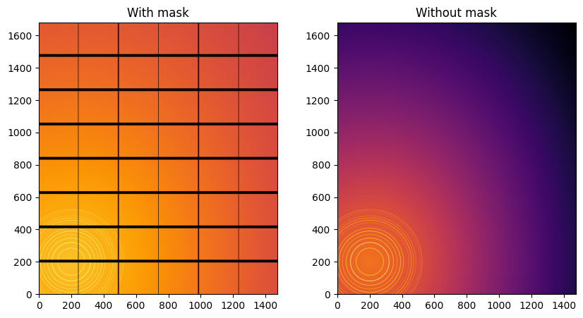
Note the aliassing effect on the displayed images.
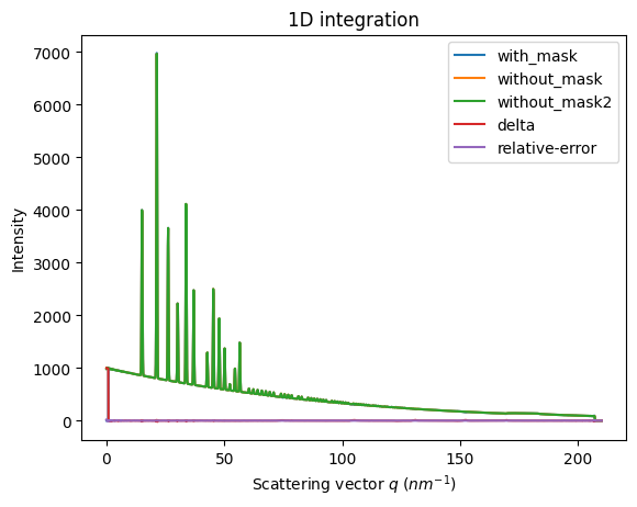
We will measure now the effect after 1D intergeration. We do not correct for polarization on purpose to highlight the defect one wishes to whipe out. We use a R-factor to describe the quality of the 1D-integrated signal.
kwargs = {"npt":2000, "unit":"q_nm^-1", "method":("full", "histogram", "cython"), "radial_range":(0,210)}
wo = ai.integrate1d(img_nomask, **kwargs)
wo2 = ai.integrate1d(img_nomask2, **kwargs)
wm = ai.integrate1d(img, mask=mask, **kwargs)
ax = jupyter.plot1d(wm , label="with_mask")
ax.plot(*wo, label="without_mask")
ax.plot(*wo2, label="without_mask2")
ax.plot(wo.radial, wo.intensity-wm.intensity, label="delta")
ax.plot(wo.radial, wo.intensity-wo2.intensity, label="relative-error")
ax.legend()
print("Between masked and non masked image R= %s"%pyFAI.utils.mathutil.rwp(wm,wo))
print("Between two different non-masked images R'= %s"%pyFAI.utils.mathutil.rwp(wo2,wo))
Between masked and non masked image R= 5.67251189999345
Between two different non-masked images R'= 0.21425939989908654
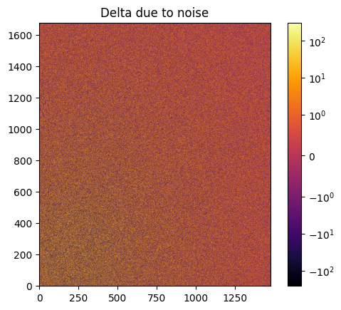
# Effect of the noise on the delta image
fig, ax = subplots()
jupyter.display(img=img_nomask-img_nomask2, label="Delta due to noise", ax=ax)
ax.figure.colorbar(ax.images[0])
<matplotlib.colorbar.Colorbar at 0x7fdc8a70ba10>
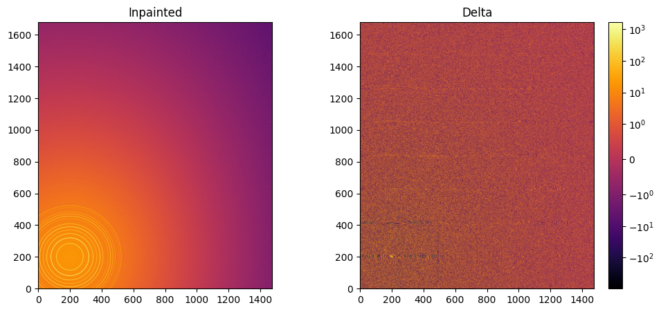
Inpainting#
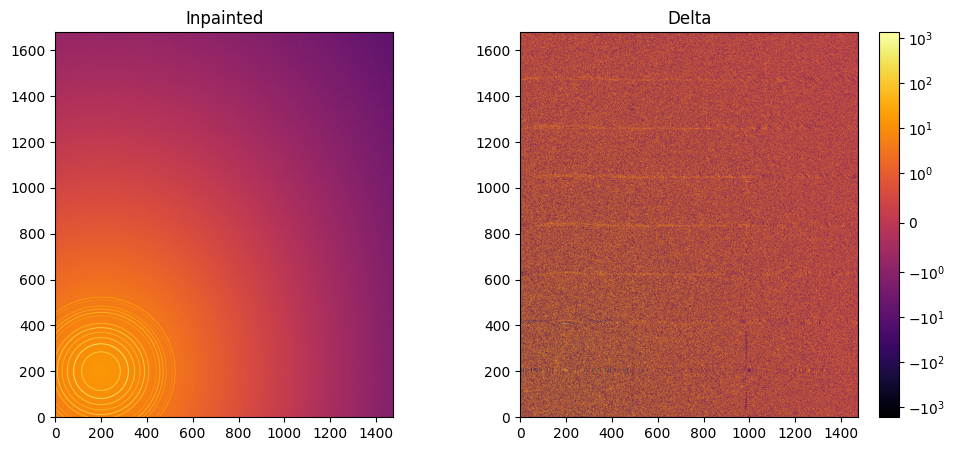
This part describes how to paint the missing pixels for having a “natural-looking image”. The delta image contains the difference with the original image
#Inpainting:
inpainted = ai.inpainting(img, mask=mask,
                          method=("no", "histogram", "cython"),
                          poissonian=True, grow_mask=3)
fig, ax = subplots(1, 2, figsize=(12,5))
jupyter.display(img=inpainted, label="Inpainted", ax=ax[0])
jupyter.display(img=img_nomask-inpainted, label="Delta", ax=ax[1])
ax[1].figure.colorbar(ax[1].images[0]);
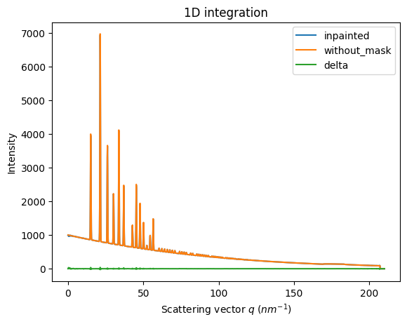
# Comparison of the inpained image with the original one:
wm = ai.integrate1d(inpainted, **kwargs)
wo = ai.integrate1d(img_nomask, **kwargs)
ax = jupyter.plot1d(wm , label="inpainted")
ax.plot(*wo, label="without_mask")
ax.plot(wo.radial, wo.intensity-wm.intensity, label="delta")
ax.legend()
print("R= %s"%pyFAI.utils.mathutil.rwp(wm,wo))
R= 0.6141101036121835

One can see by zooming in that the main effect on inpainting is a broadening of the signal in the inpainted region. This could (partially) be adressed by increasing the number of radial bins used in the inpainting.
Benchmarking and optimization of the parameters#
The parameter set depends on the detector, the experiment geometry and the type of signal on the detector. Finer detail require finer slicing.
#Basic benchmarking of execution time for default options:
%timeit inpainted = ai.inpainting(img, mask=mask)
128 ms ± 8.42 ms per loop (mean ± std. dev. of 7 runs, 1 loop each)
wo = ai.integrate1d(img_nomask, **kwargs)
R_best = numpy.finfo("float32").max
best = {}
for m in (("no", "csc", "cython"), ("bbox", "csc","cython"), ("full", "csc","cython")):
    for k in (512, 1024, 2048, 4096):
        ai.reset()
        for i in (0, 1, 2, 4, 8):
            inpainted = ai.inpainting(img, mask=mask, poissonian=True, method=m, npt_rad=k, grow_mask=i)
            wm = ai.integrate1d(inpainted, **kwargs)
            R = pyFAI.utils.mathutil.rwp(wm,wo)
            if R<R_best:
                R_best = R
                best={"method":m,
                      "npt_rad":k,
                      "grow_mask":i}
            print(f"method: {m} npt_rad={k} grow={i}; R= {R:.3f}")
print("Best configuration:", best)
method: ('no', 'csc', 'cython') npt_rad=512 grow=0; R= 2.303
method: ('no', 'csc', 'cython') npt_rad=512 grow=1; R= 0.809
method: ('no', 'csc', 'cython') npt_rad=512 grow=2; R= 0.514
method: ('no', 'csc', 'cython') npt_rad=512 grow=4; R= 0.471
method: ('no', 'csc', 'cython') npt_rad=512 grow=8; R= 0.428
method: ('no', 'csc', 'cython') npt_rad=1024 grow=0; R= 2.500
method: ('no', 'csc', 'cython') npt_rad=1024 grow=1; R= 0.872
method: ('no', 'csc', 'cython') npt_rad=1024 grow=2; R= 0.680
method: ('no', 'csc', 'cython') npt_rad=1024 grow=4; R= 0.628
method: ('no', 'csc', 'cython') npt_rad=1024 grow=8; R= 0.299
method: ('no', 'csc', 'cython') npt_rad=2048 grow=0; R= 2.749
method: ('no', 'csc', 'cython') npt_rad=2048 grow=1; R= 1.178
method: ('no', 'csc', 'cython') npt_rad=2048 grow=2; R= 1.038
method: ('no', 'csc', 'cython') npt_rad=2048 grow=4; R= 0.903
method: ('no', 'csc', 'cython') npt_rad=2048 grow=8; R= 0.645
method: ('no', 'csc', 'cython') npt_rad=4096 grow=0; R= 2.678
method: ('no', 'csc', 'cython') npt_rad=4096 grow=1; R= 1.206
method: ('no', 'csc', 'cython') npt_rad=4096 grow=2; R= 1.189
method: ('no', 'csc', 'cython') npt_rad=4096 grow=4; R= 1.155
method: ('no', 'csc', 'cython') npt_rad=4096 grow=8; R= 1.008
method: ('bbox', 'csc', 'cython') npt_rad=512 grow=0; R= 0.477
method: ('bbox', 'csc', 'cython') npt_rad=512 grow=1; R= 0.448
method: ('bbox', 'csc', 'cython') npt_rad=512 grow=2; R= 0.430
method: ('bbox', 'csc', 'cython') npt_rad=512 grow=4; R= 0.424
method: ('bbox', 'csc', 'cython') npt_rad=512 grow=8; R= 0.429
method: ('bbox', 'csc', 'cython') npt_rad=1024 grow=0; R= 0.311
method: ('bbox', 'csc', 'cython') npt_rad=1024 grow=1; R= 0.283
method: ('bbox', 'csc', 'cython') npt_rad=1024 grow=2; R= 0.279
method: ('bbox', 'csc', 'cython') npt_rad=1024 grow=4; R= 0.270
method: ('bbox', 'csc', 'cython') npt_rad=1024 grow=8; R= 0.272
method: ('bbox', 'csc', 'cython') npt_rad=2048 grow=0; R= 0.250
method: ('bbox', 'csc', 'cython') npt_rad=2048 grow=1; R= 0.236
method: ('bbox', 'csc', 'cython') npt_rad=2048 grow=2; R= 0.227
method: ('bbox', 'csc', 'cython') npt_rad=2048 grow=4; R= 0.226
method: ('bbox', 'csc', 'cython') npt_rad=2048 grow=8; R= 0.224
method: ('bbox', 'csc', 'cython') npt_rad=4096 grow=0; R= 0.239
method: ('bbox', 'csc', 'cython') npt_rad=4096 grow=1; R= 0.225
method: ('bbox', 'csc', 'cython') npt_rad=4096 grow=2; R= 0.234
method: ('bbox', 'csc', 'cython') npt_rad=4096 grow=4; R= 0.242
method: ('bbox', 'csc', 'cython') npt_rad=4096 grow=8; R= 0.233
method: ('full', 'csc', 'cython') npt_rad=512 grow=0; R= 0.485
method: ('full', 'csc', 'cython') npt_rad=512 grow=1; R= 0.436
method: ('full', 'csc', 'cython') npt_rad=512 grow=2; R= 0.432
method: ('full', 'csc', 'cython') npt_rad=512 grow=4; R= 0.426
method: ('full', 'csc', 'cython') npt_rad=512 grow=8; R= 0.437
method: ('full', 'csc', 'cython') npt_rad=1024 grow=0; R= 0.303
method: ('full', 'csc', 'cython') npt_rad=1024 grow=1; R= 0.270
method: ('full', 'csc', 'cython') npt_rad=1024 grow=2; R= 0.279
method: ('full', 'csc', 'cython') npt_rad=1024 grow=4; R= 0.270
method: ('full', 'csc', 'cython') npt_rad=1024 grow=8; R= 0.284
method: ('full', 'csc', 'cython') npt_rad=2048 grow=0; R= 1.057
method: ('full', 'csc', 'cython') npt_rad=2048 grow=1; R= 1.097
method: ('full', 'csc', 'cython') npt_rad=2048 grow=2; R= 0.867
method: ('full', 'csc', 'cython') npt_rad=2048 grow=4; R= 0.661
method: ('full', 'csc', 'cython') npt_rad=2048 grow=8; R= 0.728
method: ('full', 'csc', 'cython') npt_rad=4096 grow=0; R= 0.936
method: ('full', 'csc', 'cython') npt_rad=4096 grow=1; R= 0.921
method: ('full', 'csc', 'cython') npt_rad=4096 grow=2; R= 0.921
method: ('full', 'csc', 'cython') npt_rad=4096 grow=4; R= 0.963
method: ('full', 'csc', 'cython') npt_rad=4096 grow=8; R= 0.729
Best configuration: {'method': ('bbox', 'csc', 'cython'), 'npt_rad': 2048, 'grow_mask': 8}
#Inpainting, best solution found:
ai.reset()
%time inpainted = ai.inpainting(img, mask=mask, poissonian=True, **best)
fig, ax = subplots(1, 2, figsize=(12, 5))
jupyter.display(img=inpainted, label="Inpainted", ax=ax[0])
jupyter.display(img=img_nomask-inpainted, label="Delta", ax=ax[1])
ax[1].figure.colorbar(ax[1].images[0]);
CPU times: user 2.67 s, sys: 90.6 ms, total: 2.76 s
Wall time: 1.05 s
# Comparison of the inpained image with the original one:
wm = ai.integrate1d(inpainted, **kwargs)
wo = ai.integrate1d(img_nomask, **kwargs)
ax = jupyter.plot1d(wm , label="inpainted")
ax.plot(*wo, label="without_mask")
ax.plot(wo.radial, wo.intensity-wm.intensity, label="delta")
ax.legend()
print("R= %s"%pyFAI.utils.mathutil.rwp(wm,wo))
R= 0.22645810604437674
Conclusion#
Inpainting is one of the only solution to fill up the gaps in detector when Fourier analysis is needed. This tutorial explains basically how this is possible using the pyFAI library and how to optimize the parameter set for inpainting. The result may greatly vary with detector position and tilt and the kind of signal (amorphous or more spotty).
print(f"Execution time: {time.perf_counter()-start_time:.3f} s")
Execution time: 66.415 s