Integration with Python#
This cookbook explains you how to perform azimuthal integration using the Python interpreter. It is divided in two parts, the first part uses purely Python while the second uses some advanced features of the Jupyter notebook.
We will re-use the same files as in the other tutorials.
Performing azimuthal integration with pyFAI of a bunch of images#
To be able to perform the azimuthal integration of some images, one needs:
The diffraction images themselves, in this example they are stored as EDF files
The geometry of the experimental setup as obtained from the calibration and stored as a PONI-file
other files like flat-field, dark current images or detector distortion file (spline-file).
Image file: http://www.silx.org/pub/pyFAI/cookbook/calibration/Eiger4M_Al2O3_13.45keV.edf
Geometry file: http://www.silx.org/pub/pyFAI/cookbook/calibration/alpha-Al2O3.poni
The calibration has been performed in the previous cookbook.
Basic usage of pyFAI#
To perform azimuthal averaging, one can use pyFAI to load the geometry and FabIO to read the image:
# This cell is just to download the files to perform the analysis:
import time
import shutil, os
from silx.resources import ExternalResources

t0 = time.perf_counter()
os.environ["PYOPENCL_COMPILER_OUTPUT"] = "0"
downloader = ExternalResources("pyFAI", "http://www.silx.org/pub/pyFAI/cookbook/calibration/", "PYFAI_DATA")
image_file = downloader.getfile("Eiger4M_Al2O3_13.45keV.edf")
poni_file = downloader.getfile("alpha-Al2O3.poni")

print("image_file:", image_file)
print("poni_file:", poni_file)

# Copy all files locally
shutil.copy(poni_file, ".")
shutil.copy(image_file, ".")
# clean-up files from previous run:
for result in ('integrated.edf', "integrated.dat", "Eiger4M_Al2O3_13.45keV.dat"):
    if os.path.exists(result):
        os.unlink(result)

os.listdir()
image_file: /tmp/pyFAI_testdata_kieffer/Eiger4M_Al2O3_13.45keV.edf
poni_file: /tmp/pyFAI_testdata_kieffer/alpha-Al2O3.poni
['calib-gui',
 'Eiger4M_Al2O3_13.45keV.edf',
 'pyFAI-calib_notebook.png',
 'alpha-Al2O3.poni',
 'index.rst',
 'pyFAI-integrate.png',
 'integration_with_the_gui.rst',
 'F_K4320T_Cam43_30012013_distorsion.spline',
 'calibration_with_jupyter.ipynb',
 'Integration_with_the_GUI.ipynb',
 '.ipynb_checkpoints',
 'integration_with_python.ipynb',
 'jupyter.poni',
 'calib-cli',
 'integration_with_scripts.ipynb']
import pyFAI, fabio
print("pyFAI version:", pyFAI.version)
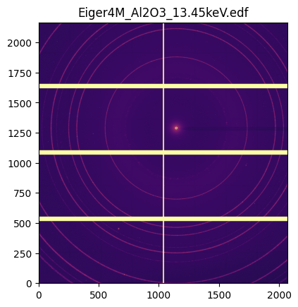
img = fabio.open("Eiger4M_Al2O3_13.45keV.edf")
print("Image:", img)
ai = pyFAI.load("alpha-Al2O3.poni")
print("\nIntegrator: \n", ai)
pyFAI version: 2025.12.0
Image: <fabio.edfimage.EdfImage object at 0x7f53f34c1550>

Integrator:
 Detector Eiger 4M	 PixelSize= 75µm, 75µm	 BottomRight (3)
Wavelength= 0.921816 Å
SampleDetDist= 1.625467e-01 m	PONI= 9.636511e-02, 8.600623e-02 m	rot1=0.002605  rot2=0.000641  rot3=0.000000 rad
DirectBeamDist= 162.547 mm	Center: x=1141.104, y=1286.257 pix	Tilt= 0.154° tiltPlanRotation= 166.178° λ= 0.922Å
Azimuthal averaging using pyFAI#
One needs first to retrieve the image as a numpy array. This allows to use other libraries than FabIO for image reading, for example HDF5 files.
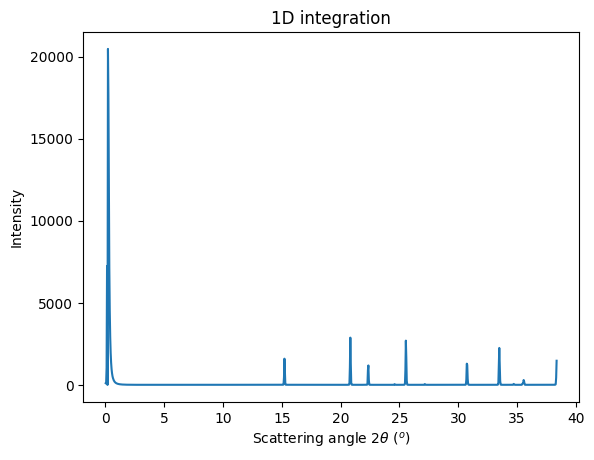
This shows how to perform the azimuthal integration of one image over 1000 bins:
img_array = img.data
print("img_array:", type(img_array), img_array.shape, img_array.dtype)
mask = img_array>4e9

res = ai.integrate1d_ng(img_array,
                        1000,
                        mask=mask,
                        unit="2th_deg",
                        filename="integrated.dat")
img_array: <class 'numpy.ndarray'> (2167, 2070) float32
Note: There are 2 mandatory parameters for this method: the 2D-numpy array with the image and the number of bins. In addition, we specified the name of the file where to save the data and the unit for performing the integration.
There are many other options of integrate1d. The difference between the legacy and the ng flavor is mostly on the way error is propagated:
help(ai.integrate1d_ng)
Help on method integrate1d in module pyFAI.integrator.azimuthal:

integrate1d(
    data,
    npt,
    *,
    filename=None,
    correctSolidAngle=True,
    variance=None,
    error_model=None,
    radial_range=None,
    azimuth_range=None,
    mask=None,
    dummy=None,
    delta_dummy=None,
    polarization_factor=None,
    dark=None,
    flat=None,
    absorption=None,
    method=('bbox', 'csr', 'cython'),
    unit=q_nm^-1,
    safe=True,
    normalization_factor=1.0,
    metadata=None
) method of pyFAI.integrator.azimuthal.AzimuthalIntegrator instance
    Calculate the azimuthal integration (1d) of a 2D image.

    Multi algorithm implementation (tries to be bullet proof), suitable for SAXS, WAXS, ... and much more
    Takes extra care of normalization and performs proper variance propagation.

    :param ndarray data: 2D array from the Detector/CCD camera
    :param int npt: number of points in the output pattern
    :param str filename: output filename in 2/3 column ascii format
    :param bool correctSolidAngle: correct for solid angle of each pixel if True
    :param ndarray variance: array containing the variance of the data.
    :param str error_model: When the variance is unknown, an error model can be given: "poisson" (variance = I), "azimuthal" (variance = (I-<I>)^2)
    :param radial_range: The lower and upper range of the radial unit. If not provided, range is simply (min, max). Values outside the range are ignored.
    :type radial_range: (float, float), optional
    :param azimuth_range: The lower and upper range of the azimuthal angle in degree. If not provided, range is simply (min, max). Values outside the range are ignored.
    :type azimuth_range: (float, float), optional
    :param ndarray mask: array with  0 for valid pixels, all other are masked (static mask)
    :param float dummy: value for dead/masked pixels (dynamic mask)
    :param float delta_dummy: precision for dummy value
    :param float polarization_factor: polarization factor between -1 (vertical) and +1 (horizontal).
           0 for circular polarization or random,
           None for no correction,
           True for using the former correction
    :param ndarray dark: dark noise image
    :param ndarray flat: flat field image
    :param ndarray absorption: absorption correction image
    :param IntegrationMethod method: IntegrationMethod instance or 3-tuple with (splitting, algorithm, implementation)
    :param Unit unit: Output units, can be "q_nm^-1" (default), "2th_deg", "r_mm" for now.
    :param bool safe: Perform some extra checks to ensure LUT/CSR is still valid. False is faster.
    :param float normalization_factor: Value of a normalization monitor
    :param metadata: JSON serializable object containing the metadata, usually a dictionary.
    :param ndarray absorption: detector absorption
    :return: Integrate1dResult namedtuple with (q,I,sigma) +extra information in it.
The result file contains the integrated data with some headers as shown:
with open("integrated.dat") as f:
    for i in range(50):
        print(f.readline().strip())
# {
#     "poni_version": 2.1,
#     "dist": 0.16254673947902704,
#     "poni1": 0.09636511239091199,
#     "poni2": 0.08600622810318177,
#     "rot1": 0.0026048269580961157,
#     "rot2": 0.0006408875619633374,
#     "rot3": 7.381054962294179e-11,
#     "detector": "Eiger4M",
#     "detector_config": {
#         "pixel1": 7.5e-05,
#         "pixel2": 7.5e-05,
#         "orientation": 3
#     },
#     "wavelength": 9.218156017338309e-11
# }
# Mask applied: user provided
# Dark current applied: False
# Flat field applied: False
# Polarization factor: None
# Normalization factor: 1.0
# --> integrated.dat
#2th_deg        I
1.919453e-02    1.069847e+02
5.758360e-02    1.369709e+02
9.597267e-02    1.055195e+03
1.343617e-01    7.239173e+03
1.727508e-01    0.000000e+00
2.111399e-01    2.046833e+04
2.495289e-01    1.767060e+04
2.879180e-01    1.170923e+04
3.263071e-01    7.144739e+03
3.646961e-01    4.495782e+03
4.030852e-01    2.918516e+03
4.414743e-01    1.955727e+03
4.798633e-01    1.355407e+03
5.182524e-01    9.685643e+02
5.566415e-01    7.158437e+02
5.950305e-01    5.435187e+02
6.334196e-01    4.240506e+02
6.718087e-01    3.373720e+02
7.101977e-01    2.713135e+02
7.485868e-01    2.221988e+02
7.869759e-01    1.840064e+02
8.253649e-01    1.547038e+02
8.637540e-01    1.308537e+02
9.021431e-01    1.118036e+02
9.405321e-01    9.608984e+01
9.789212e-01    8.361955e+01
1.017310e+00    7.308739e+01
Azimuthal regrouping using pyFAI#
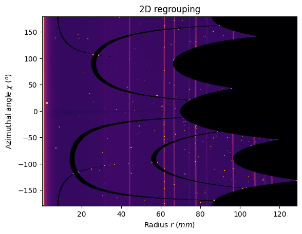
This option is similar to the integration but performs N integrations on various azimuthal angle (chi) sections of the space. It is also named “caking” in Fit2D.
The azimuthal regrouping of an image over 500 radial bins in 360 angular steps (of 1 degree) can be performed like this:
res2 = ai.integrate2d_ng(img_array,
                         500, 360,
                         unit="r_mm",
                         filename="integrated.edf")
cake = fabio.open("integrated.edf")
print(cake.header)
print("cake:", type(cake.data), cake.data.shape, cake.data.dtype)
{
  "EDF_DataBlockID": "0.Image.Psd",
  "EDF_BinarySize": "720000",
  "EDF_HeaderSize": "1024",
  "ByteOrder": "LowByteFirst",
  "DataType": "FloatValue",
  "Dim_1": "500",
  "Dim_2": "360",
  "Image": "0",
  "HeaderID": "EH:000000:000000:000000",
  "Size": "720000",
  "Engine": "None",
  "r_mm_min": "0.12896015039433978",
  "r_mm_max": "128.83119024394543",
  "chi_deg_min": "179.50004447175695",
  "has_mask_applied": "from detector",
  "has_dark_correction": "False",
  "has_flat_correction": "False",
  "polarization_factor": "None",
  "normalization_factor": "1.0"
}
cake: <class 'numpy.ndarray'> (360, 500) float32
From this, it is trivial to perform a loop and integrate many images.
Attention: The AzimuthalIntegrator object (called ai here) is rather large and costly to initialize. The best practice is to create it once and to use it many times, like this:
import glob, os

all_images = glob.glob("Eiger4M_*.edf")
ai = pyFAI.load("alpha-Al2O3.poni")

for one_image in all_images:
    fimg = fabio.open(one_image)
    dest = os.path.splitext(one_image)[0] + ".dat"
    ai.integrate1d_ng(fimg.data,
                   1000,
                   unit="2th_deg",
                   filename=dest)
Using some advanced features of Jupyter Notebooks#
Jupyter notebooks offer some advanced visualization features, especially when used with matplotlib and pyFAI. Unfortunately, the example shown hereafter will not work properly in normal Python scipts.
Initialization of the notebook for matplotlib integration:#
from pyFAI.gui import jupyter
Visualization of different types of results previously calculated#
jupyter.display(img.data, label=img.filename);
jupyter.plot1d(res);
jupyter.plot2d(res2);
Conclusion#
This cookbook explains the basic usage of pyFAI as a Python library for azimuthal integration and simple visualization in the Jupyter notebook.
print(f"Total execution time: {time.perf_counter() - t0 :6.3f} s")
Total execution time: 11.287 s