Calibration of a diffraction setup using Jupyter notebooks#
This notebook presents a very simple GUI for doing the calibration of diffraction setup within the Jupyter-Lab or Jupyter-Notebook environment with Matplotlib and Ipywidgets.
It has been tested with widget and the notebook (aka nbagg) integration of matplotlib.
It requires also matplotlib.inline
Despite this is in the cookbook section, this tutorial requires advanced Python programming knowledge and some good understanding of PyFAI.
This tutorial is also available as a video:
#Video of this tutorial
#Skip to 7:55 in you already know jupyter notebook and you are just interested in the calibration.
from IPython.display import Video

Video("http://www.silx.org/pub/pyFAI/video/Calibration_Jupyter.mp4", width=800)
The basic idea is to port directly the original pyFAI-calib tool which was done with matplotlib into the Jupyter notebooks. Most credits go Philipp Hans for the adaptation of the origin PeakPicker class to Jupyter.
The PeakPicker widget has been refactored and the Calibration tool adapted for the notebook usage. Several external tools were used with the following version:
for lib in ["jupyterlab", "notebook", "matplotlib", "matplotlib_inline", "ipympl", "ipywidgets"]:
    mod = __import__(lib)
    print(f"{lib:18s}:   {mod.__version__}")
jupyterlab        :   4.4.10
notebook          :   7.4.5
matplotlib        :   3.10.8
matplotlib_inline :   0.1.7
ipympl            :   0.9.7
ipywidgets        :   8.1.5
# The notebook interface (nbagg) is needed in jupyter-notebook while the widget is recommended for jupyer lab
# %matplotlib nbagg
# %matplotlib widget
# For the integration in the documentation, one uses `inline` to capture figures.
# %matplotlib inline

import json
import pyFAI
import pyFAI.test.utilstest
import fabio
from matplotlib.pyplot import subplots
from pyFAI.gui import jupyter
from pyFAI.gui.jupyter.calib import Calibration

print(f"PyFAI version {pyFAI.version}")
WARNING:pyFAI.gui.matplotlib:Matplotlib already loaded with backend `module://ipympl.backend_nbagg`, setting its backend to `QtAgg` may not work!
PyFAI version 2025.12.0
# Some parameters like the wavelength, the calibrant and the diffraction image:
wavelength = 1e-10
pilatus = pyFAI.detector_factory("Pilatus1M")
AgBh = pyFAI.calibrant.CALIBRANT_FACTORY("AgBh")
AgBh.wavelength = wavelength

#load some test data (requires an internet connection)
img = fabio.open(pyFAI.test.utilstest.UtilsTest.getimage("Pilatus1M.edf")).data
%matplotlib inline
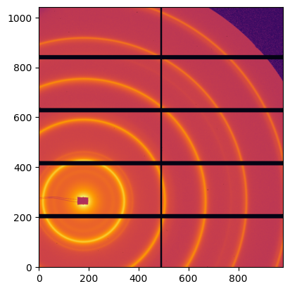
# Simply display the scattering image:
jupyter.display(img);
%matplotlib widget
calib = Calibration(img, calibrant=AgBh, wavelength=wavelength, detector=pilatus)
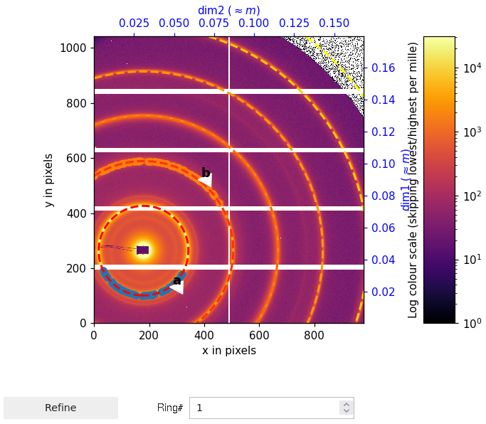
# This displays the calibration widget:
# 1. Set the ring number (0-based value), below the plot
# 2. Pick the ring by right-clicking with the mouse on the image.
# 3. Restart at 1. for at least a second ring
# 4. Click refine to launch the calibration.
# Here is a screenshot of the previous widget, since it is not recoreded inside the notebook itself.
from IPython.display import Image
Image(filename='pyFAI-calib_notebook.png')
# This is the calibrated geometry:
gr = calib.geoRef
print(gr)
print(f"{calib.fixed}")
print(f"Cost function: {gr.chi2()}")
Detector Pilatus 1M	 PixelSize= 172µm, 172µm	 BottomRight (3)
Wavelength= 1.000000 Å
SampleDetDist= 1.635096e+00 m	PONI= 4.344199e-02, 3.192409e-02 m	rot1=0.000613  rot2=0.001213  rot3=0.000000 rad
DirectBeamDist= 1635.098 mm	Center: x=179.775, y=264.100 pix	Tilt= 0.078° tiltPlanRotation= 116.824° λ= 1.000Å
Fixed parameters: rot3, wavelength.
Cost function: 1.5989928144588604e-07
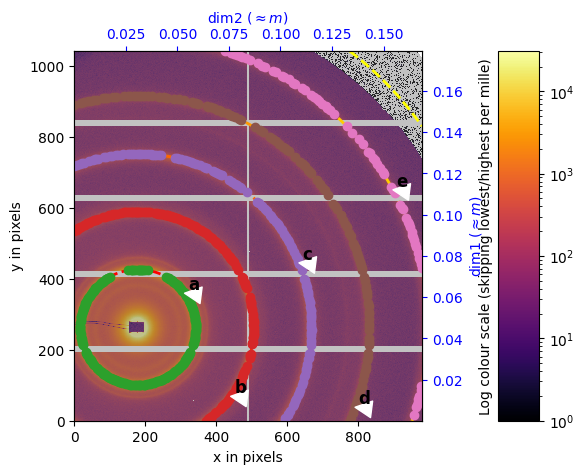
# re-extract all control points using the "massif" algorithm
calib.extract_cpt()
# remove the last ring since it is outside the flight-tube
calib.remove_grp(lbl="f")
# Switch back to `inline` mode to capture the last plot
%matplotlib inline
calib.peakPicker.widget.fig.show()
#Those are some control points: the last column indicates the ring number
calib.geoRef.data[::100]
array([[3.59534671e+02, 3.10521346e+02, 0.00000000e+00],
       [1.84940919e+02, 3.66357618e+01, 0.00000000e+00],
       [2.54000610e+02, 3.41987457e+02, 0.00000000e+00],
       [1.89004883e+02, 4.96961090e+02, 1.00000000e+00],
       [4.63965703e+02, 6.25654486e+02, 2.00000000e+00],
       [3.80974764e+02, 6.53535562e+02, 2.00000000e+00],
       [6.04969131e+02, 7.35380761e+02, 3.00000000e+00],
       [1.01704657e+03, 4.94472961e+02, 4.00000000e+00]])
# This is the geometry with all rings defined:
gr = calib.geoRef
print(gr)
print(f"{calib.fixed}")
print(f"Cost function: {gr.chi2()}")
Detector Pilatus 1M	 PixelSize= 172µm, 172µm	 BottomRight (3)
Wavelength= 1.000000 Å
SampleDetDist= 1.635096e+00 m	PONI= 4.344199e-02, 3.192409e-02 m	rot1=0.000613  rot2=0.001213  rot3=0.000000 rad
DirectBeamDist= 1635.098 mm	Center: x=179.775, y=264.100 pix	Tilt= 0.078° tiltPlanRotation= 116.824° λ= 1.000Å
Fixed parameters: rot3, wavelength.
Cost function: 9.528178201413747e-07
# Geometry refinement with some constrains: SAXS mode
# Here we enforce all rotation to be null and fit again the model:

gr.rot1 = gr.rot2 = gr.rot3 = 0
gr.refine3(fix=["rot1", "rot2", "rot3", "wavelength"])
print(gr)
print(f"Cost function = {gr.chi2()}")
Detector Pilatus 1M	 PixelSize= 172µm, 172µm	 BottomRight (3)
Wavelength= 1.000000 Å
SampleDetDist= 1.635075e+00 m	PONI= 4.541940e-02, 3.093455e-02 m	rot1=0.000000  rot2=0.000000  rot3=0.000000 rad
DirectBeamDist= 1635.075 mm	Center: x=179.852, y=264.066 pix	Tilt= 0.000° tiltPlanRotation= 0.000° λ= 1.000Å
Cost function = 9.335748363699462e-07
gr.save("jupyter.poni")
print(json.dumps(gr.get_config(), indent=2))
{
  "poni_version": 2.1,
  "dist": 1.6350748395798615,
  "poni1": 0.04541939819801539,
  "poni2": 0.030934547269883487,
  "rot1": 0.0,
  "rot2": 0.0,
  "rot3": 0.0,
  "detector": "Pilatus1M",
  "detector_config": {
    "pixel1": 0.000172,
    "pixel2": 0.000172,
    "orientation": 3
  },
  "wavelength": 1e-10
}
# Create a "normal" azimuthal integrator (without fitting capabilities from the geometry-refinement object)
ai = pyFAI.load(gr)
ai
Detector Pilatus 1M	 PixelSize= 172µm, 172µm	 BottomRight (3)
Wavelength= 1.000000 Å
SampleDetDist= 1.635075e+00 m	PONI= 4.541940e-02, 3.093455e-02 m	rot1=0.000000  rot2=0.000000  rot3=0.000000 rad
DirectBeamDist= 1635.075 mm	Center: x=179.852, y=264.066 pix	Tilt= 0.000° tiltPlanRotation= 0.000° λ= 1.000Å
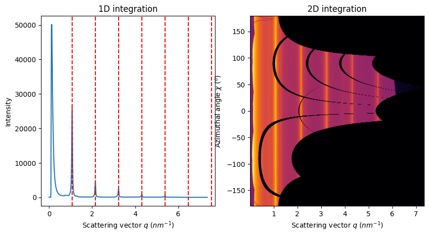
# Display the integrated data to validate the calibration.
fig, ax = subplots(1, 2, figsize=(10, 5))
jupyter.plot1d(ai.integrate1d(img, 1000),  calibrant=AgBh, ax=ax[0])
jupyter.plot2d(ai.integrate2d(img, 1000),  calibrant=AgBh, ax=ax[1])
ax[1].set_title("2D integration");
Conclusion#
This short notebook shows how to interact with a calibration image to pick some control-point from the Debye-Scherrer ring and to perform the calibration of the experimental setup.