Deconvolution of the Thickness effect#
This is the third part of this long journey in the thickness of the silicon sensor of the Pilatus detector: after characterizing the precise position of the Pilatus-1M on the goniometer of ID28 we noticed there are some discrepancies in the ring position and peak width as function of the position on the detector. In a second time the thickness of the detector was modeled and allowed us to define a sparse-matrix which represent the bluring of the signal with a point-spread function which actually depends on the position of the detector. This convolution can be revereted using techniques developped for inverse problems. Two pseudo-inversion algorithm have been tested, either limiting least-squares errors or with poissonian constrains.
We will now correct the images of the first notebook called “goniometer” with the sparse matrix calculated in the second one (called “raytracing”) and check if the pick-width is less chaotic and if peaks are actually thinner.
# %matplotlib widget
%matplotlib inline
# use `widget` instead of `inline` for better user-exeperience. `inline` allows to store plots into notebooks.
import os
import time
start_time = time.perf_counter()
import numpy
import fabio, pyFAI
from os.path import basename
from pyFAI.gui import jupyter
from pyFAI.calibrant import get_calibrant
from silx.resources import ExternalResources
from matplotlib.pyplot import subplots
from matplotlib.lines import Line2D
from ipywidgets import interact, interactive, fixed, interact_manual
import ipywidgets as widgets
downloader = ExternalResources("thick", "http://www.silx.org/pub/pyFAI/testimages")
all_files = downloader.getdir("gonio_ID28.tar.bz2")
for afile in all_files:
    print(basename(afile))
gonio_ID28
det130_g45_0001p.npt
det130_g0_0001p.cbf
det130_g17_0001p.npt
det130_g0_0001p.npt
det130_g45_0001p.cbf
det130_g17_0001p.cbf
from scipy.sparse import save_npz, load_npz, csr_matrix, csc_matrix, linalg
#Saved in notebook called "raytracing"
csr = load_npz("csr.npz")
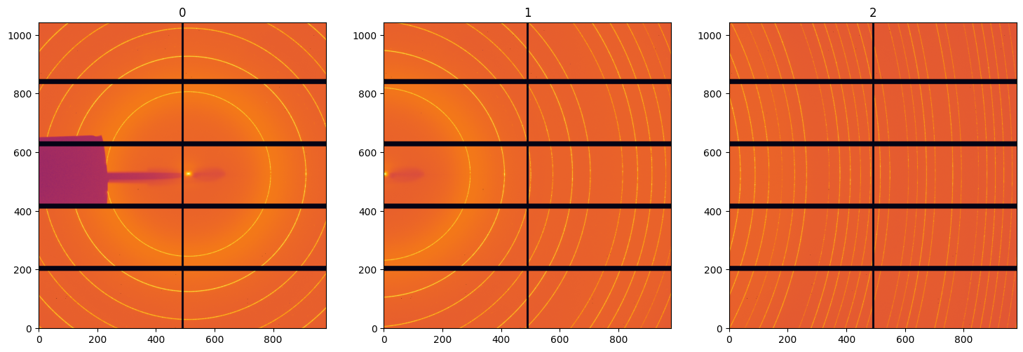
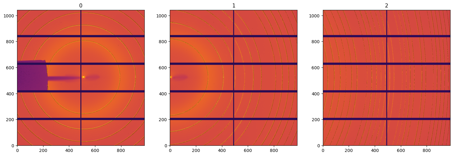
# Display all images as acquired
mask = numpy.load("mask.npy")
images = [fabio.open(i).data for i in sorted(all_files) if i.endswith("cbf")]

fig, ax = subplots(1, 3, figsize=(18, 6))
for i, img in enumerate(images):
    jupyter.display(img, ax=ax[i], label=str(i))
# Display all images once they have been corrected with least-squares minimization

fig, ax = subplots(1, 3, figsize=(18, 6))

msk = numpy.where(mask)
for i, img in enumerate(images):
    fl = img.astype("float32")
    fl[msk] = 0.0 # set masked values to 0, negative values could induce errors
    bl = fl.ravel()
    res = linalg.lsmr(csr.T, bl)
    print(res[1:])
    cor = res[0].reshape(img.shape)
    jupyter.display(cor, ax=ax[i], label=str(i))
/users/kieffer/.venv/py313/lib/python3.13/site-packages/scipy/sparse/linalg/_isolve/lsmr.py:407: RuntimeWarning: overflow encountered in cast
  condA = max(maxrbar, rhotemp) / min(minrbar, rhotemp)
/users/kieffer/.venv/py313/lib/python3.13/site-packages/scipy/sparse/linalg/_isolve/lsmr.py:406: RuntimeWarning: overflow encountered in cast
  minrbar = min(minrbar, rhobarold)
(1, 21, 75.26544884972343, np.float32(13.849053), 1.8677121626358506, np.float32(3.6550646), np.float64(42781250.69143017))
(1, 22, 53.96384651698693, np.float32(9.754348), 1.9135295515208164, np.float32(3.7043958), np.float64(37022792.71982042))
(1, 22, 35.13108144746531, np.float32(6.550181), 1.9074681251632473, np.float32(3.6570237), np.float64(15773856.309523012))
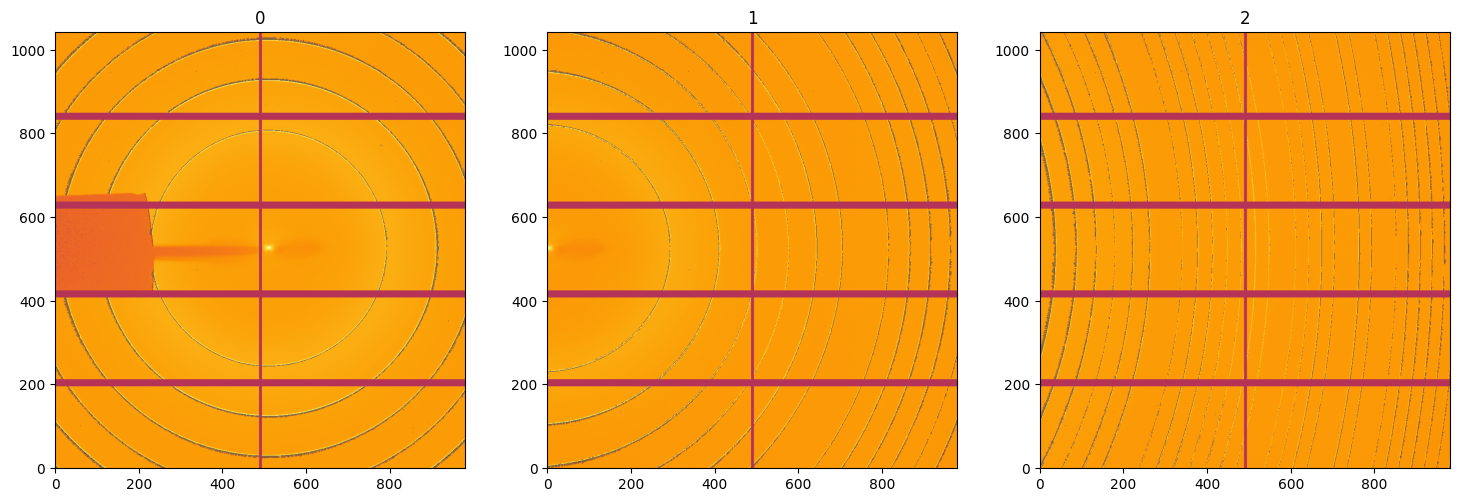
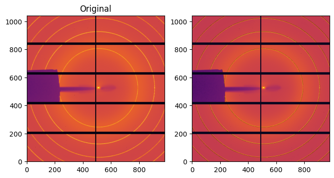
It turns out the deconvolution is not that straight forwards and creates some negative wobbles near the rings. This phenomenon is well known in inverse methods which provide a damping factor to limit the effect. This damping factor needs to be adjusted manually to avoid this.
img = images[0]
fl = img.astype("float32")
fl[msk] = 0.0 # set masked values to 0
blured = fl.ravel()
fig, ax = subplots(1, 2, figsize=(8, 4))
im0 = ax[0].imshow(numpy.arcsinh(fl), cmap="inferno")
im1 = ax[1].imshow(numpy.arcsinh(fl), cmap="inferno")
ax[0].set_title("Original")
ax[1].set_title("Deconvolved")
def deconvol(damp):
    res = linalg.lsmr(csr.T, blured, damp=damp, x0=blured)
    restored = res[0].reshape(mask.shape)
    im1.set_data(numpy.arcsinh(restored))
    print("Number of negative pixels: %i"%(restored<0).sum())


interactive_plot = widgets.interactive(deconvol, damp=(0, 5.0))
display(interactive_plot)
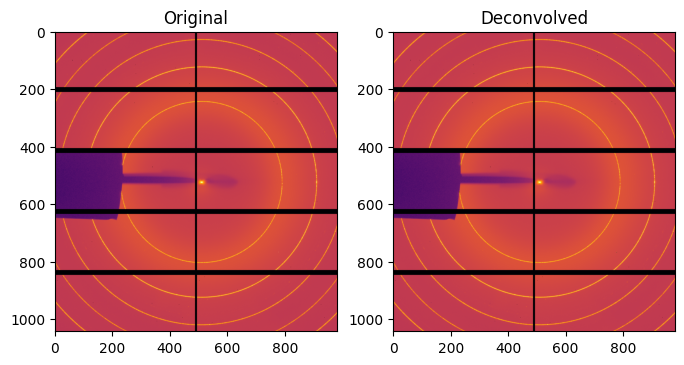
#selection of the damping factor which provides no negative signal:
tot_neg = 100
damp = 0
while tot_neg>0:
    damp += 0.1
    tot_neg = 0
    deconvoluted = []
    for i, img in enumerate(images):
        fl = img.astype("float32")
        fl[msk] = 0.0 # set masked values to 0
        bl = fl.ravel()
        res = linalg.lsmr(csr.T, bl, damp=damp)
        neg=(res[0]<0).sum()
        print(i, damp, neg, res[1:])
        tot_neg += neg
        deconvoluted.append(res[0].reshape(img.shape))
print("damp:",damp)
0 0.1 12692 (2, 19, 4133473.5091587612, np.float32(5.8514624), 1.7794778273321978, np.float32(3.1927035), np.float64(39976785.698201895))
1 0.1 12064 (2, 19, 3593526.4842869933, np.float32(6.2880054), 1.782841891314785, np.float32(3.2799995), np.float64(34907677.668833956))
2 0.1 17211 (2, 20, 1509973.7649808293, np.float32(2.2622302), 1.8206537278878563, np.float32(3.3229382), np.float64(14487949.98921174))
0 0.2 11687 (2, 14, 7598567.143457593, np.float32(6.7594767), 1.5346120398753222, np.float32(2.623072), np.float64(34011019.8480814))
1 0.2 10679 (2, 14, 6670629.014180683, np.float32(6.338296), 1.539546135370012, np.float32(2.649661), np.float64(30233577.65135094))
2 0.2 14892 (2, 14, 2736967.6316883187, np.float32(3.6475914), 1.5335937002515274, np.float32(2.6504686), np.float64(12064126.117767107))
0 0.30000000000000004 9718 (2, 11, 10238577.360395856, np.float32(5.802144), 1.3675464703825244, np.float32(2.2106025), np.float64(27764325.396945275))
1 0.30000000000000004 9091 (2, 11, 9072908.593784282, np.float32(5.128135), 1.3728888951195541, np.float32(2.1932144), np.float64(25063134.622167915))
2 0.30000000000000004 12327 (2, 11, 3652108.1665425804, np.float32(2.8298466), 1.3655459330909248, np.float32(2.1788592), np.float64(9730736.902739085))
0 0.4 8287 (2, 9, 12173170.037708893, np.float64(5.727362432226614), 1.245863124827177, np.float64(1.8485235115350627), np.float64(22342146.027704857))
1 0.4 7593 (2, 9, 10864701.70638546, np.float64(5.094353622798936), 1.2494695968653682, np.float64(1.848945545625006), np.float64(20382306.973381624))
2 0.4 9895 (2, 9, 4315740.777631027, np.float64(2.7700191668041168), 1.2394794719791953, np.float64(1.8474985620334985), np.float64(7777852.933821111))
0 0.5 6792 (2, 8, 13575136.695301248, np.float64(3.2819479221254166), 1.1784467930555054, np.float64(1.598254886342562), np.float64(17965896.9320742))
1 0.5 5955 (2, 8, 12177831.213735664, np.float64(2.940783554544499), 1.1814135120392153, np.float64(1.6063030508188345), np.float64(16503028.034637759))
2 0.5 7428 (2, 8, 4793882.649636383, np.float64(1.5437294140832172), 1.1706062569571416, np.float64(1.6017532628414737), np.float64(6228179.950032172))
0 0.6 5262 (2, 7, 14594803.28524327, np.float64(3.613804641012908), 1.1057209495542177, np.float64(1.411617090942349), np.float64(14540087.291315816))
1 0.6 4312 (2, 7, 13139593.623746458, np.float64(3.1464994113292404), 1.1106878222728596, np.float64(1.4101376482218178), np.float64(13416709.377460856))
2 0.6 5210 (2, 7, 5140356.30327638, np.float64(1.6222813548247186), 1.097957420437241, np.float64(1.4093829547158898), np.float64(5026362.962932841))
0 0.7 3870 (2, 6, 15345002.133048056, np.float64(7.024831487400084), 1.0295961585507463, np.float64(1.2532853755901223), np.float64(11884919.528255012))
1 0.7 2995 (2, 6, 13850363.124408964, np.float64(6.130426754746088), 1.0347061618238402, np.float64(1.2560658492175487), np.float64(11000269.918408293))
2 0.7 3486 (2, 6, 5394615.969240544, np.float64(3.094859234173296), 1.0210158256327995, np.float64(1.2529863769316822), np.float64(4100335.6460272553))
0 0.7999999999999999 2621 (2, 6, 15905434.177499492, np.float64(2.0477623039099373), 1.0295961585507463, np.float64(1.1253981893059006), np.float64(9824933.826364845))
1 0.7999999999999999 1949 (2, 6, 14382915.824495899, np.float64(1.7912194544760907), 1.0347061618238402, np.float64(1.1273899638107003), np.float64(9113047.589470306))
2 0.7999999999999999 2185 (2, 6, 5584208.540078377, np.float64(0.8960980029364765), 1.0210158256327995, np.float64(1.125257619214536), np.float64(3384728.375595408))
0 0.8999999999999999 1631 (2, 5, 16331092.206976132, np.float64(8.656857430003512), 0.9475860997437712, np.float64(1.0423800983474896), np.float64(8215743.083816755))
1 0.8999999999999999 1226 (2, 5, 14788224.35965244, np.float64(7.711004419618497), 0.9546095433848871, np.float64(1.0475690595426306), np.float64(7632166.222569134))
2 0.8999999999999999 1319 (2, 5, 5728010.11089549, np.float64(3.8761211971709795), 0.9384434085828889, np.float64(1.042427814363324), np.float64(2827295.0792616066))
0 0.9999999999999999 988 (2, 5, 16659766.197224312, np.float64(3.581387314142279), 0.9475860997437712, np.float64(1.0346948461413814), np.float64(6946438.49047354))
1 0.9999999999999999 750 (2, 5, 15101639.670068745, np.float64(3.1964954305117446), 0.9546095433848871, np.float64(1.0389986325789056), np.float64(6460357.065037574))
2 0.9999999999999999 812 (2, 5, 5838931.284802746, np.float64(1.597825799061224), 0.9384434085828889, np.float64(1.0350726122949256), np.float64(2388513.4761898927))
0 1.0999999999999999 565 (2, 5, 16917578.64039506, np.float64(1.5739698187798625), 0.9475860997437712, np.float64(1.0288879669921127), np.float64(5934264.8102116315))
1 1.0999999999999999 442 (2, 5, 15347745.516513832, np.float64(1.4070640616994885), 0.9546095433848871, np.float64(1.0325117183466226), np.float64(5523765.367132678))
2 1.0999999999999999 502 (2, 5, 5925868.338094836, np.float64(0.7003166841164902), 0.9384434085828889, np.float64(1.0294255592283825), np.float64(2039169.6617480833))
0 1.2 323 (2, 5, 17122796.764230706, np.float64(0.7303610912169005), 0.9475860997437712, np.float64(1.0244047976543667), np.float64(5118092.304335518))
1 1.2 251 (2, 5, 15543802.145704396, np.float64(0.6537542745787962), 0.9546095433848871, np.float64(1.0274954076007683), np.float64(4767228.567021776))
2 1.2 288 (2, 5, 5995025.55689959, np.float64(0.3242819228532609), 0.9384434085828889, np.float64(1.025010343960121), np.float64(1757817.2016205743))
0 1.3 192 (2, 4, 17288368.74191142, np.float64(9.277956273162046), 0.8553444062185472, np.float64(1.021103595483284), np.float64(4452765.006043024))
1 1.3 152 (2, 4, 15702080.546424238, np.float64(8.33251409580545), 0.8655803324608607, np.float64(1.0226359760153911), np.float64(4149694.058423326))
2 1.3 196 (2, 4, 6050794.108126477, np.float64(4.209409026391478), 0.845721273249541, np.float64(1.0215009495815173), np.float64(1528685.2218142992))
0 1.4000000000000001 123 (2, 4, 17423612.477967475, np.float64(5.4101094198572754), 0.8553444062185472, np.float64(1.0182690915952812), np.float64(3904752.657226766))
1 1.4000000000000001 94 (2, 4, 15831429.882265577, np.float64(4.864658367177063), 0.8655803324608607, np.float64(1.0196077801552133), np.float64(3640516.802461945))
2 1.4000000000000001 129 (2, 4, 6096329.135919276, np.float64(2.4516025003665756), 0.845721273249541, np.float64(1.0186699857354138), np.float64(1340101.2387562862))
0 1.5000000000000002 72 (2, 4, 17535332.995910197, np.float64(3.2546288030660313), 0.8553444062185472, np.float64(1.0159644106984893), np.float64(3448954.6305916617))
1 1.5000000000000002 59 (2, 4, 15938321.810991844, np.float64(2.9294011112097302), 0.8655803324608607, np.float64(1.0171433178676148), np.float64(3216666.1417178693))
2 1.5000000000000002 89 (2, 4, 6133930.869054721, np.float64(1.4733858190495206), 0.845721273249541, np.float64(1.0163560416583746), np.float64(1183348.6251927307))
0 1.6000000000000003 51 (2, 4, 17628570.562137015, np.float64(2.013723840062398), 0.8553444062185472, np.float64(1.0140665608317612), np.float64(3066401.029994724))
1 1.6000000000000003 39 (2, 4, 16027559.256917303, np.float64(1.8139977665146603), 0.8655803324608607, np.float64(1.0151121015301459), np.float64(2860686.7433015336))
2 1.6000000000000003 51 (2, 4, 6165303.659656419, np.float64(0.9108779668362268), 0.845721273249541, np.float64(1.0144420151090383), np.float64(1051853.6819296707))
0 1.7000000000000004 39 (2, 4, 17707113.55310375, np.float64(1.2779893561377114), 0.8553444062185472, np.float64(1.0124858233279652), np.float64(2742611.8381641544))
1 1.7000000000000004 20 (2, 4, 16102751.062023122, np.float64(1.1520373070539476), 0.8655803324608607, np.float64(1.0134191090295859), np.float64(2559222.339277931))
2 1.7000000000000004 36 (2, 4, 6191725.446820809, np.float64(0.5776847342729973), 0.845721273249541, np.float64(1.0128419175282632), np.float64(940605.641784951))
0 1.8000000000000005 29 (2, 4, 17773842.97605594, np.float64(0.8299534579651535), 0.8553444062185472, np.float64(1.0111558030039607), np.float64(2466420.218955527))
1 1.8000000000000005 14 (2, 4, 16166646.75488748, np.float64(0.7485999505209011), 0.8655803324608607, np.float64(1.0119937504982242), np.float64(2301955.157639794))
2 1.8000000000000005 25 (2, 4, 6214168.611498556, np.float64(0.3749444869094572), 0.845721273249541, np.float64(1.0114913619460064), np.float64(845745.6524080619))
0 1.9000000000000006 20 (2, 4, 17830978.20056128, np.float64(0.550396135354225), 0.8553444062185472, np.float64(1.010026492688817), np.float64(2229128.97909831))
1 1.9000000000000006 9 (2, 4, 16221366.165291745, np.float64(0.496696548140879), 0.8655803324608607, np.float64(1.0107827740094226), np.float64(2080837.5216934977))
2 1.9000000000000006 14 (2, 4, 6233381.976858482, np.float64(0.24852804374691875), 0.845721273249541, np.float64(1.010341462649575), np.float64(764271.4511117352))
0 2.0000000000000004 17 (2, 4, 17880250.14086776, np.float64(0.3720460988035753), 0.8553444062185472, np.float64(1.0090693600514267), np.float64(2023899.3572654582))
1 2.0000000000000004 5 (2, 4, 16268562.52765469, np.float64(0.3358937343452035), 0.8655803324608607, np.float64(1.0097454027113322), np.float64(1889533.5107669693))
2 2.0000000000000004 8 (2, 4, 6249948.586665426, np.float64(0.1679243862165897), 0.845721273249541, np.float64(1.0093546460202234), np.float64(693824.1854699741))
0 2.1000000000000005 16 (2, 4, 17923019.00234074, np.float64(0.2559268866983994), 0.8553444062185472, np.float64(1.0082457411858023), np.float64(1845303.2982245476))
1 2.1000000000000005 5 (2, 4, 16309534.865729412, np.float64(0.2311454477087679), 0.8655803324608607, np.float64(1.008850243528441), np.float64(1723008.9939811302))
2 2.1000000000000005 2 (2, 4, 6264326.9058306785, np.float64(0.115471477781231), 0.845721273249541, np.float64(1.008501734428704), np.float64(632533.1176828115))
0 2.2000000000000006 13 (2, 3, 17960368.331006307, np.float64(13.37547968821848), 0.7527743524408553, np.float64(1.0076086951124774), np.float64(1688995.7389317702))
1 2.2000000000000006 4 (2, 3, 16345319.394383248, np.float64(11.519783398778143), 0.7645565284652346, np.float64(1.0081140149578058), np.float64(1577231.141671821))
2 2.2000000000000006 1 (2, 4, 6276881.94299203, np.float64(0.08069243180034831), 0.845721273249541, np.float64(1.0077596676333778), np.float64(578901.6709918618))
0 2.3000000000000007 10 (2, 3, 17993167.003347058, np.float64(10.342638123565022), 0.7527743524408553, np.float64(1.0069679296807355), np.float64(1551469.1964603928))
1 2.3000000000000007 2 (2, 3, 16376747.164774915, np.float64(8.910351950247227), 0.7645565284652346, np.float64(1.0074324128176644), np.float64(1448942.1441709714))
2 2.3000000000000007 1 (2, 3, 6287905.943395343, np.float64(4.432170899419076), 0.744615578453984, np.float64(1.0071894584491285), np.float64(531722.3548771262))
0 2.400000000000001 10 (2, 3, 18022117.785223894, np.float64(8.079559544756478), 0.7527743524408553, np.float64(1.0064045758584226), np.float64(1429870.2581308559))
1 2.400000000000001 1 (2, 3, 16404489.993446566, np.float64(6.962490187716206), 0.7645565284652346, np.float64(1.0068329188396352), np.float64(1335489.9890806335))
2 2.400000000000001 0 (2, 3, 6297636.392338696, np.float64(3.461743557636721), 0.744615578453984, np.float64(1.0066056350910957), np.float64(490013.5131072759))
0 2.500000000000001 9 (2, 3, 18047795.32708535, np.float64(6.371642603131994), 0.7527743524408553, np.float64(1.0059066422070477), np.float64(1321860.8040731729))
1 2.500000000000001 1 (2, 3, 16429098.080315625, np.float64(5.491978165702877), 0.7645565284652346, np.float64(1.0063028394453781), np.float64(1234700.583697366))
2 2.500000000000001 0 (2, 3, 6306265.535199845, np.float64(2.729540143609506), 0.744615578453984, np.float64(1.0060900503468608), np.float64(452970.778871565))
0 2.600000000000001 7 (2, 3, 18070670.39829039, np.float64(5.069078063071377), 0.7527743524408553, np.float64(1.005464441552724), np.float64(1225511.2513711902))
1 2.600000000000001 1 (2, 3, 16451021.598684838, np.float64(4.370144655496815), 0.7645565284652346, np.float64(1.0058319508695046), np.float64(1144778.7695522124))
2 2.600000000000001 0 (2, 3, 6313952.232653459, np.float64(2.1712284728406255), 0.744615578453984, np.float64(1.005632479157471), np.float64(419930.8090557677))
0 2.700000000000001 6 (2, 3, 18091132.46917378, np.float64(4.065895635832328), 0.7527743524408553, np.float64(1.005070025961018), np.float64(1139218.9961093825))
1 2.700000000000001 1 (2, 3, 16470634.694854613, np.float64(3.505928619109421), 0.7645565284652346, np.float64(1.0054117578064234), np.float64(1064233.2175486304))
2 2.700000000000001 0 (2, 3, 6320828.156032941, np.float64(1.7413170497866843), 0.744615578453984, np.float64(1.0052245011342302), np.float64(390342.8590504734))
0 2.800000000000001 5 (2, 3, 18109508.835611153, np.float64(3.286206279469259), 0.7527743524408553, np.float64(1.0047166619973), np.float64(1061645.175213788))
1 2.800000000000001 1 (2, 3, 16488247.907220513, np.float64(2.8340883738155824), 0.7645565284652346, np.float64(1.0050352990673026), np.float64(991817.0884230552))
2 2.800000000000001 0 (2, 3, 6327002.706297522, np.float64(1.4072366776747363), 0.744615578453984, np.float64(1.004859201253261), np.float64(363746.7835194721))
0 2.9000000000000012 4 (2, 3, 18126070.24452694, np.float64(2.675031071687997), 0.7527743524408553, np.float64(1.0043989382443677), np.float64(991664.0230839615))
1 2.9000000000000012 0 (2, 3, 16504123.597467134, np.float64(2.3073425500201297), 0.7645565284652346, np.float64(1.0046966478892585), np.float64(926482.3434292891))
2 2.9000000000000012 0 (2, 3, 6332567.218269331, np.float64(1.145398919925377), 0.744615578453984, np.float64(1.0045308809346885), np.float64(339755.8917183686))
0 3.0000000000000013 4 (2, 3, 18141046.736106444, np.float64(2.1921099444059315), 0.7527743524408553, np.float64(1.0041122186654448), np.float64(928324.4013436636))
1 3.0000000000000013 0 (2, 3, 16518480.721677039, np.float64(1.8910544886945253), 0.7645565284652346, np.float64(1.0043909687610282), np.float64(867342.7749188466))
2 3.0000000000000013 0 (2, 3, 6337598.703436642, np.float64(0.9385342425165425), 0.744615578453984, np.float64(1.0042347638508846), np.float64(318043.4807511381))
0 3.1000000000000014 2 (2, 3, 18154633.580074776, np.float64(1.807661107519573), 0.7527743524408553, np.float64(1.0038525771207), np.float64(870818.3868700183))
1 3.1000000000000014 0 (2, 3, 16531505.863016801, np.float64(1.5595946152985531), 0.7645565284652346, np.float64(1.0041141219311716), np.float64(813645.531440932))
2 3.1000000000000014 0 (2, 3, 6342163.4224892305, np.float64(0.7738707726650691), 0.744615578453984, np.float64(1.0039666686442625), np.float64(298332.18874921784))
0 3.2000000000000015 0 (2, 3, 18166996.53492667, np.float64(1.499443622395953), 0.7527743524408553, np.float64(1.0036167165326204), np.float64(818456.2782666136))
1 3.2000000000000015 0 (2, 3, 16543357.002814842, np.float64(1.2938174507826383), 0.7645565284652346, np.float64(1.0038626545721816), np.float64(764747.7493149181))
2 3.2000000000000015 0 (2, 3, 6346316.528260772, np.float64(0.6418720572430175), 0.744615578453984, np.float64(1.0037232555177158), np.float64(280385.1742481996))
damp: 3.2000000000000015
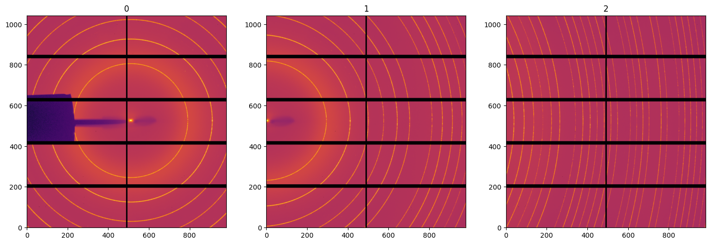
#Display deconvoluted images:
fig, ax = subplots(1, 3, figsize=(18, 6))
for i,img in enumerate(deconvoluted):
    jupyter.display(img, ax=ax[i], label=str(i))
Validation using the goniometer refinement#
At this point we are back to the initial state: can we fit the goniometer and check the width of the peaks to validate if it got better.
wavelength=0.6968e-10
calibrant = get_calibrant("LaB6")
calibrant.wavelength = wavelength
print(calibrant)

detector =  pyFAI.detector_factory("Pilatus1M")
detector.mask = mask

fimages = []
fimages.append(fabio.cbfimage.CbfImage(data=deconvoluted[0], header={"angle":0}))
fimages.append(fabio.cbfimage.CbfImage(data=deconvoluted[1], header={"angle":17}))
fimages.append(fabio.cbfimage.CbfImage(data=deconvoluted[2], header={"angle":45}))
LaB6 Calibrant with 120 reflections at wavelength 6.968e-11
def get_angle(metadata):
    """Takes the basename (like det130_g45_0001.cbf ) and returns the angle of the detector"""
    return metadata["angle"]
from pyFAI.goniometer import GeometryTransformation, GoniometerRefinement, Goniometer
from pyFAI.gui import jupyter
gonioref2d = GoniometerRefinement.sload("id28.json", pos_function=get_angle)
for idx, fimg in enumerate(fimages):
    sg = gonioref2d.new_geometry(str(idx), image=fimg.data, metadata=fimg.header, calibrant=calibrant)
    print(sg.label, "Angle:", sg.get_position())
0 Angle: 0
1 Angle: 17
2 Angle: 45
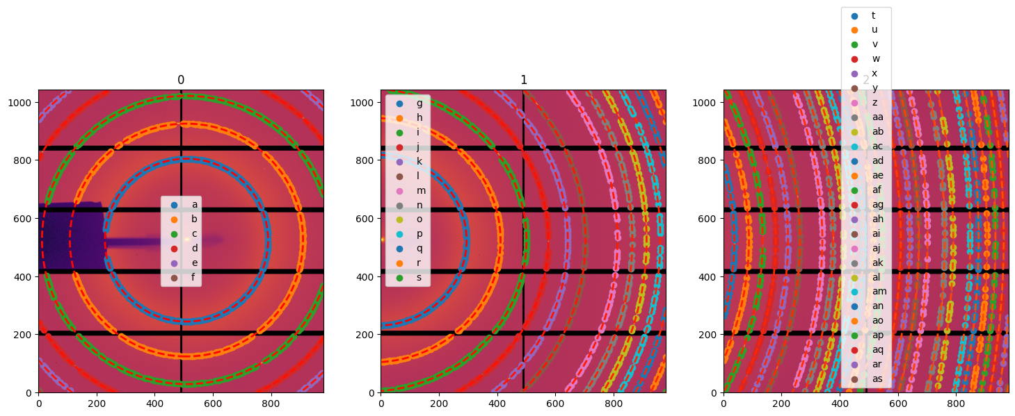
# Display the control points freshly extracted on all 3 images:
fig,ax = subplots(1,3, figsize=(18, 6))
for lbl, sg in gonioref2d.single_geometries.items():
    idx = int(lbl)
    print(sg.extract_cp())
    jupyter.display(sg=sg, ax=ax[idx])
ControlPoints instance containing 6 group of point:
LaB6 Calibrant with 120 reflections at wavelength 6.968e-11
Containing 6 groups of points:
# a ring 0: 348 points
# b ring 1: 341 points
# c ring 2: 316 points
# d ring 3: 129 points
# e ring 4: 48 points
# f ring 5: 2 points
ControlPoints instance containing 13 group of point:
LaB6 Calibrant with 120 reflections at wavelength 6.968e-11
Containing 13 groups of points:
# g ring 0: 177 points
# h ring 1: 172 points
# i ring 2: 168 points
# j ring 3: 123 points
# k ring 4: 106 points
# l ring 5: 94 points
# m ring 6: 80 points
# n ring 7: 77 points
# o ring 8: 71 points
# p ring 9: 67 points
# q ring 10: 37 points
# r ring 11: 16 points
# s ring 12: 1 points
ControlPoints instance containing 26 group of point:
LaB6 Calibrant with 120 reflections at wavelength 6.968e-11
Containing 26 groups of points:
# t ring 7: 37 points
# u ring 8: 54 points
# v ring 9: 66 points
# w ring 10: 64 points
# x ring 11: 62 points
# y ring 12: 61 points
# z ring 13: 57 points
#aa ring 14: 55 points
#ab ring 15: 55 points
#ac ring 16: 53 points
#ad ring 17: 53 points
#ae ring 18: 47 points
#af ring 19: 50 points
#ag ring 20: 49 points
#ah ring 21: 47 points
#ai ring 22: 47 points
#aj ring 23: 45 points
#ak ring 24: 45 points
#al ring 25: 43 points
#am ring 26: 43 points
#an ring 27: 42 points
#ao ring 28: 41 points
#ap ring 29: 41 points
#aq ring 30: 41 points
#ar ring 31: 19 points
#as ring 32: 3 points
#Refine the model:
gonioref2d.refine2()
Cost function before refinement: 3.315987973130784e-08
[ 2.84547625e-01  8.86548898e-02  8.93078322e-02  5.48987903e-03
  5.54613259e-03  1.74619292e-02 -2.09755151e-05]
 message: Optimization terminated successfully
 success: True
  status: 0
     fun: 1.9946473045072837e-08
       x: [ 2.844e-01  8.866e-02  8.931e-02  5.490e-03  5.547e-03
            1.746e-02 -2.063e-05]
     nit: 5
     jac: [ 8.720e-08  1.352e-06  3.213e-06 -1.022e-06  5.486e-07
           -2.758e-05 -2.541e-07]
    nfev: 49
    njev: 5
Cost function after refinement: 1.9946473045072837e-08
GonioParam(dist=np.float64(0.28437567632830285), poni1=np.float64(0.0886587466871428), poni2=np.float64(0.08930603392722097), rot1=np.float64(0.005489750983831797), rot2=np.float64(0.005546802403520394), scale1=np.float64(0.017461647689371505), scale2=np.float64(-2.0629404669706027e-05))
maxdelta on: dist (0) 0.2845476247369457 --> 0.28437567632830285
array([ 2.84375676e-01,  8.86587467e-02,  8.93060339e-02,  5.48975098e-03,
        5.54680240e-03,  1.74616477e-02, -2.06294047e-05])
# Create a MultiGeometry integrator from the refined geometry:
angles = []
dimages = []
for sg in gonioref2d.single_geometries.values():
angles.append(sg.get_position())
dimages.append(sg.image)
multigeo = gonioref2d.get_mg(angles)
multigeo.radial_range=(0, 63)
print(multigeo)
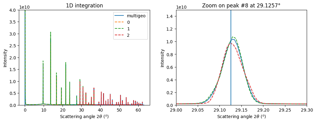
# Integrate the whole set of images in a single run:
res_mg = multigeo.integrate1d(dimages, 10000)
fig, ax = subplots(1, 2, figsize=(12,4))
ax0 = jupyter.plot1d(res_mg, label="multigeo", ax=ax[0])
ax1 = jupyter.plot1d(res_mg, label="multigeo", ax=ax[1])
# Let's focus on the inner most ring on the image taken at 45°:
for lbl, sg in gonioref2d.single_geometries.items():
ai = gonioref2d.get_ai(sg.get_position())
img = sg.image * ai.dist * ai.dist / ai.pixel1 / ai.pixel2
res = ai.integrate1d(img, 5000, unit="2th_deg", method="splitpixel")
ax0.plot(*res, "--", label=lbl)
ax1.plot(*res, "--", label=lbl)
ax1.set_xlim(29,29.3)
ax0.set_ylim(0, 4e10)
ax1.set_ylim(0, 1.5e10)
p8tth = numpy.rad2deg(calibrant.get_2th()[7])
ax1.set_title("Zoom on peak #8 at %.4f°"%p8tth)
l = Line2D([p8tth, p8tth], [0, 2e10])
ax1.add_line(l)
ax0.legend()
ax1.legend().remove()
MultiGeometry integrator with 3 geometries on (0, 63) radial range ((2th_deg, chi_deg)) and (-180, 180) azimuthal range (deg)
#Peak FWHM

from scipy.interpolate import interp1d
from scipy.optimize import bisect

def calc_fwhm(integrate_result, calibrant):
    "calculate the tth position and FWHM for each peak"
    delta = integrate_result.intensity[1:] - integrate_result.intensity[:-1]
    maxima = numpy.where(numpy.logical_and(delta[:-1]>0, delta[1:]<0))[0]
    minima = numpy.where(numpy.logical_and(delta[:-1]<0, delta[1:]>0))[0]
    maxima += 1
    minima += 1
    tth = []
    FWHM = []
    for tth_rad in calibrant.get_2th():
        tth_deg = tth_rad*integrate_result.unit.scale
        if (tth_deg<=integrate_result.radial[0]) or (tth_deg>=integrate_result.radial[-1]):
            continue
        idx_theo = abs(integrate_result.radial-tth_deg).argmin()
        id0_max = abs(maxima-idx_theo).argmin()
        id0_min = abs(minima-idx_theo).argmin()
        I_max = integrate_result.intensity[maxima[id0_max]]
        I_min = integrate_result.intensity[minima[id0_min]]
        tth_maxi = integrate_result.radial[maxima[id0_max]]
        I_thres = (I_max + I_min)/2.0
        if minima[id0_min]>maxima[id0_max]:
            if id0_min == 0:
                min_lo = integrate_result.radial[0]
            else:
                min_lo = integrate_result.radial[minima[id0_min-1]]
            min_hi = integrate_result.radial[minima[id0_min]]
        else:
            if id0_min == len(minima) -1:
                min_hi = integrate_result.radial[-1]
            else:
                min_hi = integrate_result.radial[minima[id0_min+1]]
            min_lo = integrate_result.radial[minima[id0_min]]

        f = interp1d(integrate_result.radial, integrate_result.intensity-I_thres)
        tth_lo = bisect(f, min_lo, tth_maxi)
        tth_hi = bisect(f, tth_maxi, min_hi)
        FWHM.append(tth_hi-tth_lo)
        tth.append(tth_deg)
    return tth, FWHM

fig, ax = subplots()
ax.plot(*calc_fwhm(res_mg, calibrant), "o", label="multi")
for lbl, sg in gonioref2d.single_geometries.items():
    ai = gonioref2d.get_ai(sg.get_position())
    img = sg.image * ai.dist * ai.dist / ai.pixel1 / ai.pixel2
    res = ai.integrate1d(img, 5000, unit="2th_deg", method="splitpixel")
    t,w = calc_fwhm(res, calibrant=calibrant)
    ax.plot(t, w,"-o", label=lbl)
ax.set_title("Peak shape as function of the angle")
ax.set_xlabel(res_mg.unit.label)
ax.legend()
pass
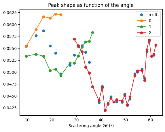
Conclusion on deconvolution using least-squares:#
The results do not look enhanced compared to the initial fit: neither the peak position, nor the FWHM looks enhanced. Maybe there is an error somewhere.
Pseudo inverse with positivitiy constrain and poissonian noise (MLEM)#
MLEM has provided similar results to least-sqares pseudo inversion with positivity constrains and the assumption of poisson noise.
# Function used for ONE MLEM iteration:

def iterMLEM_scipy(F, M, R):
    "Perform one iteration"
    #res = F * (R.T.dot(M))/R.dot(F)# / M.sum(axis=-1)
    norm = 1/R.T.dot(numpy.ones_like(F))
    cor = R.T.dot(M/R.dot(F))
    #print(norm.shape, F.shape, cor.shape)
    res = norm * F * cor
    res[numpy.isnan(res)] = 1.0
    return res
def deconv_MLEM(csr, data, thres=0.2, maxiter=1e6):
    R = csr.T
    msk = data<0
    img = data.astype("float32")
    img[msk] = 0.0 # set masked values to 0, negative values could induce errors
    M = img.ravel()
    #F0 = numpy.random.random(data.size)#M#
    F0 = R.T.dot(M)
    F1 = iterMLEM_scipy(F0, M, R)
    delta = abs(F1-F0).max()
    for i in range(int(maxiter)):
        if delta<thres:
            break
        F2 = iterMLEM_scipy(F1, M, R)
        delta = abs(F1-F2).max()
        if i%100==0:
            print(i, delta)
        F1 = F2
        i+=1
    print(i, delta)
    return F2.reshape(img.shape)
raw = images[0]
cor = deconv_MLEM(csr, images[0], maxiter=2000)

#Display one corrected image:
fig, ax = subplots(1, 2, figsize=(8,4))
im0 = ax[0].imshow(numpy.arcsinh(raw), origin="lower", cmap="inferno")
im1 = ax[1].imshow(numpy.arcsinh(cor), origin="lower", cmap="inferno")
ax[0].set_title("Original")
pass
/tmp/ipykernel_826929/1273356881.py:6: RuntimeWarning: divide by zero encountered in divide
  norm = 1/R.T.dot(numpy.ones_like(F))
/tmp/ipykernel_826929/1273356881.py:7: RuntimeWarning: invalid value encountered in divide
  cor = R.T.dot(M/R.dot(F))
/tmp/ipykernel_826929/1273356881.py:9: RuntimeWarning: invalid value encountered in multiply
  res = norm * F * cor
0 251794.0
100 148.49365
200 35.322266
300 14.653809
400 8.575684
500 4.866699
600 2.8061523
700 1.6494141
800 1.081543
900 0.859375
1000 0.6972656
1100 0.5598755
1200 0.4494629
1300 0.375
1400 0.375
1500 0.375
1600 0.375
1700 0.375
1800 0.375
1900 0.375
2000 0.5
deconvoluted = []
for i, img in enumerate(images):
    cor = deconv_MLEM(csr, img, maxiter=2000)
    deconvoluted.append(cor)
/tmp/ipykernel_826929/1273356881.py:6: RuntimeWarning: divide by zero encountered in divide
  norm = 1/R.T.dot(numpy.ones_like(F))
/tmp/ipykernel_826929/1273356881.py:7: RuntimeWarning: invalid value encountered in divide
  cor = R.T.dot(M/R.dot(F))
/tmp/ipykernel_826929/1273356881.py:9: RuntimeWarning: invalid value encountered in multiply
  res = norm * F * cor
0 251794.0
100 148.49365
200 35.322266
300 14.653809
400 8.575684
500 4.866699
600 2.8061523
700 1.6494141
800 1.081543
900 0.859375
1000 0.6972656
1100 0.5598755
1200 0.4494629
1300 0.375
1400 0.375
1500 0.375
1600 0.375
1700 0.375
1800 0.375
1900 0.375
2000 0.5
0 377996.12
100 144.25
200 47.4375
300 26.302734
400 11.446533
500 6.041748
600 3.6617432
700 2.434204
800 1.7261963
900 1.2827148
1000 0.9880371
1100 0.7825928
1200 0.633667
1300 0.522522
1400 0.4375
1500 0.375
1600 0.31793213
1700 0.2750244
1800 0.375
1900 0.25
2000 0.375
0 134638.19
100 62.65576
200 53.17383
300 29.029297
400 20.746094
500 11.878174
600 7.713379
700 5.283203
800 3.79187
900 2.826538
1000 2.1732178
1100 1.7137451
1200 1.3798828
1300 1.3125
1400 1.4619141
1500 1.5429688
1600 1.5449219
1700 1.4765625
1800 1.359375
1900 1.2089844
2000 1.0507812
# # Re-normalization
# for img, cor in zip(images, deconvoluted):
#     msk = img>=0
#     ratio = img[msk].sum()/cor[msk].sum()
#     print(ratio)
#     cor *= ratio
#     cor[numpy.logical_not(msk)] = -1
fig, ax = subplots(1, 3, figsize=(18, 6))
for i,img in enumerate(deconvoluted):
    jupyter.display(img, ax=ax[i], label=str(i))
wavelength=0.6968e-10
calibrant = get_calibrant("LaB6")
calibrant.wavelength = wavelength
print(calibrant)

detector =  pyFAI.detector_factory("Pilatus1M")
detector.mask = mask

fimages = []
fimages.append(fabio.cbfimage.CbfImage(data=deconvoluted[0], header={"angle":0}))
fimages.append(fabio.cbfimage.CbfImage(data=deconvoluted[1], header={"angle":17}))
fimages.append(fabio.cbfimage.CbfImage(data=deconvoluted[2], header={"angle":45}))
LaB6 Calibrant with 120 reflections at wavelength 6.968e-11
def get_angle(metadata):
    """Takes the basename (like det130_g45_0001.cbf ) and returns the angle of the detector"""
    return metadata["angle"]
gonioref2d = GoniometerRefinement.sload("id28.json", pos_function=get_angle)
for idx, fimg in enumerate(fimages):
    sg = gonioref2d.new_geometry(str(idx), image=fimg.data, metadata=fimg.header, calibrant=calibrant)
    print(sg.label, "Angle:", sg.get_position())
0 Angle: 0
1 Angle: 17
2 Angle: 45
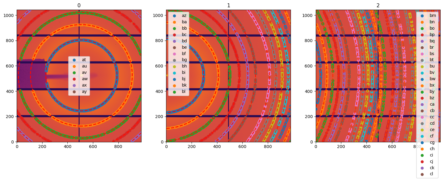
# Display the control points freshly extracted on all 3 images:

fig,ax = subplots(1,3, figsize=(18, 6))
for lbl, sg in gonioref2d.single_geometries.items():
    idx = int(lbl)
    print(sg.extract_cp())
    jupyter.display(sg=sg, ax=ax[idx])
ControlPoints instance containing 6 group of point:
LaB6 Calibrant with 120 reflections at wavelength 6.968e-11
Containing 6 groups of points:
#at ring 0: 348 points
#au ring 1: 341 points
#av ring 2: 316 points
#aw ring 3: 129 points
#ax ring 4: 48 points
#ay ring 5: 2 points
ControlPoints instance containing 13 group of point:
LaB6 Calibrant with 120 reflections at wavelength 6.968e-11
Containing 13 groups of points:
#az ring 0: 177 points
#ba ring 1: 172 points
#bb ring 2: 168 points
#bc ring 3: 123 points
#bd ring 4: 106 points
#be ring 5: 94 points
#bf ring 6: 80 points
#bg ring 7: 77 points
#bh ring 8: 71 points
#bi ring 9: 67 points
#bj ring 10: 37 points
#bk ring 11: 16 points
#bl ring 12: 1 points
ControlPoints instance containing 26 group of point:
LaB6 Calibrant with 120 reflections at wavelength 6.968e-11
Containing 26 groups of points:
#bm ring 7: 37 points
#bn ring 8: 54 points
#bo ring 9: 66 points
#bp ring 10: 64 points
#bq ring 11: 62 points
#br ring 12: 61 points
#bs ring 13: 57 points
#bt ring 14: 55 points
#bu ring 15: 55 points
#bv ring 16: 53 points
#bw ring 17: 53 points
#bx ring 18: 47 points
#by ring 19: 50 points
#bz ring 20: 49 points
#ca ring 21: 47 points
#cb ring 22: 47 points
#cc ring 23: 45 points
#cd ring 24: 45 points
#ce ring 25: 43 points
#cf ring 26: 43 points
#cg ring 27: 42 points
#ch ring 28: 41 points
#ci ring 29: 41 points
#cj ring 30: 41 points
#ck ring 31: 19 points
#cl ring 32: 3 points
gonioref2d.refine2()
Cost function before refinement: 3.0443041509132135e-08
[ 2.84547625e-01  8.86548898e-02  8.93078322e-02  5.48987903e-03
  5.54613259e-03  1.74619292e-02 -2.09755151e-05]
 message: Optimization terminated successfully
 success: True
  status: 0
     fun: 2.0789019367078762e-08
       x: [ 2.844e-01  8.866e-02  8.931e-02  5.489e-03  5.547e-03
            1.746e-02 -2.107e-05]
     nit: 7
     jac: [ 1.075e-06 -1.303e-06  1.359e-06 -2.401e-07 -1.351e-07
            1.043e-05  5.330e-06]
    nfev: 65
    njev: 7
Cost function after refinement: 2.0789019367078762e-08
GonioParam(dist=np.float64(0.28440045866449903), poni1=np.float64(0.0886594227461097), poni2=np.float64(0.08930697713127102), rot1=np.float64(0.005488813672713926), rot2=np.float64(0.005546557980359355), scale1=np.float64(0.017461927975594916), scale2=np.float64(-2.106889253806264e-05))
maxdelta on: dist (0) 0.2845476247369457 --> 0.28440045866449903
array([ 2.84400459e-01,  8.86594227e-02,  8.93069771e-02,  5.48881367e-03,
        5.54655798e-03,  1.74619280e-02, -2.10688925e-05])
#Create a MultiGeometry integrator from the refined geometry:
angles = []
dimages = []
for sg in gonioref2d.single_geometries.values():
angles.append(sg.get_position())
dimages.append(sg.image)
multigeo = gonioref2d.get_mg(angles)
multigeo.radial_range=(0, 63)
print(multigeo)
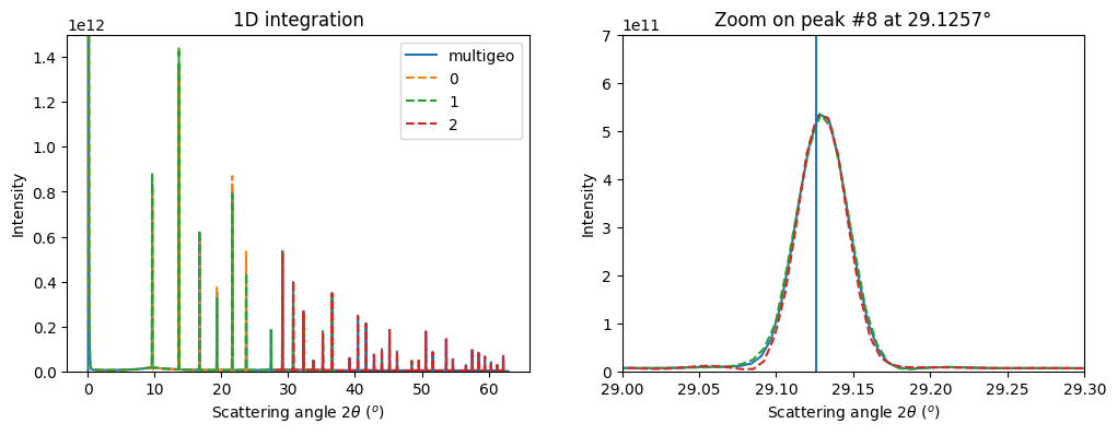
# Integrate the whole set of images in a single run:
res_mg = multigeo.integrate1d(dimages, 10000)
fig, ax = subplots(1, 2, figsize=(12, 4))
ax0 = jupyter.plot1d(res_mg, label="multigeo", ax=ax[0])
ax1 = jupyter.plot1d(res_mg, label="multigeo", ax=ax[1])
# Let's focus on the inner most ring on the image taken at 45°:
for lbl, sg in gonioref2d.single_geometries.items():
ai = gonioref2d.get_ai(sg.get_position())
img = sg.image * ai.dist * ai.dist / ai.pixel1 / ai.pixel2
res = ai.integrate1d(img, 5000, unit="2th_deg", method=("full", "histogram","cython"))
ax0.plot(*res, "--", label=lbl)
ax1.plot(*res, "--", label=lbl)
ax1.set_xlim(29,29.3)
ax0.set_ylim(0, 1.5e12)
ax1.set_ylim(0, 7e11)
p8tth = numpy.rad2deg(calibrant.get_2th()[7])
ax1.set_title("Zoom on peak #8 at %.4f°"%p8tth)
l = Line2D([p8tth, p8tth], [0, 2e12])
ax1.add_line(l)
ax0.legend()
ax1.legend().remove()
MultiGeometry integrator with 3 geometries on (0, 63) radial range ((2th_deg, chi_deg)) and (-180, 180) azimuthal range (deg)
# FWHM plot
fig, ax = subplots()
ax.plot(*calc_fwhm(res_mg, calibrant), "o", label="multi")
for lbl, sg in gonioref2d.single_geometries.items():
    ai = gonioref2d.get_ai(sg.get_position())
    img = sg.image * ai.dist * ai.dist / ai.pixel1 / ai.pixel2
    res = ai.integrate1d(img, 5000, unit="2th_deg", method=("full", "histogram","cython"))
    t,w = calc_fwhm(res, calibrant=calibrant)
    ax.plot(t, w,"-o", label=lbl)
ax.set_title("Peak shape as function of the angle")
ax.set_xlabel(res_mg.unit.label)
ax.legend()
pass
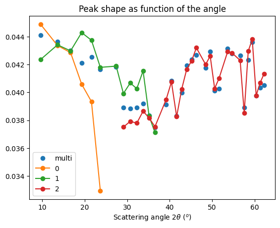
Conclusion#
The MLEM deconvolution provided thinner peak (~10% thinner), the fit for the geometry is in the same level of quality. Deconvoluted images are more noisy and there is a ring with zeros shadowing close to the highest intensities.
For the future (i.e. TODO):
Properly treat masked pixel as invalid ones
Provide some regulatization to induce less moise.
Implement MLEM in a more efficient way (cython, OpenCL, …)
print(f"Total execution time: {time.perf_counter()-start_time:.3f} s")
Total execution time: 137.471 s