
Writing NXdata#
This tutorial explains how to write a NXdata group into a HDF5 file.
A basic knowledge of the HDF5 file format, including understanding the concepts of group, dataset and attribute, is a prerequisite for this tutorial. You should also be able to read a Python script using the h5py library to write HDF5 data. You can find some information on these topics at the beginning of the Getting started with silx.io tutorial.
Definitions#
NeXus Data Format#
NeXus is a common data format for neutron, x-ray, and muon science. It is being developed as an international standard by scientists and programmers representing major scientific facilities in order to facilitate greater cooperation in the analysis and visualization of neutron, x-ray, and muon data.
It uses the HDF5 format, adding additional rules and structure to help people and software understand how to read a data file.
The name of a group in a NeXus data file can be any string of characters, but it must have a NX_class attribute defining a *class type*.
Examples of such classes are:
NXroot: root group of the file (may be implicit, if the NX_class attribute is omitted)
NXentry: describes a measurement; it is mandatory that there is at least one group of this type in the NeXus file
NXsample: contains information pertaining to the sample, such as its chemical composition, mass, and environment variables (temperature, pressure, magnetic field, etc.)
NXinstrument: encapsulates all the instrumental information that might be relevant to a measurement
NXdata: describes the plottable data and related dimension scales
You can find all the specifications about the NeXus format on the nexusformat.org website. The rest of this tutorial will focus exclusively on NXdata.
NXdata groups#
NXdata describes the plottable data and related dimension scales.
It is mandatory that there is at least one NXdata group in each NXentry group. Note that the variable and data can be defined with different names. The signal and axes attributes of the group define which items are plottable data and which are dimension scales, respectively.
In the case of a curve, for instance, you would have a 1D signal dataset (y values) and optionally another 1D signal of identical size as axis (x values). In the case of an image, you would have a 2D dataset as signal and optionally two 1D datasets to scale the X and Y axes.
A NXdata group should define all the information needed to provide a sensible plot, including axis labels and a plot title. It can also include additional metadata such as standard deviations of data values, or errors an axes.
Note
The NXdata specification evolved slightly over the course of time. The complete documentation for the *NXdata* class mentions older rules that you will probably have to take into account if you intend to write a program that reads NeXus files.
If you only need to write such files and only need to read back files you have yourself written, you should adhere to the most recent rules. We will only mention these most recent specifications in this tutorial.
Main elements in a NXdata group#
Signal#
The @signal attribute of the NXdata group provides the name of a dataset containing the plottable data. The name of this dataset can be freely chosen by the writer.
This signal dataset may have a @long_name attribute, that can be used as an axis label (e.g. for the Y axis of a curve) or a plot title (e.g. for an image).
Axes#
The @axes attributes of the NXdata group provides a list of names of datasets to be used as dimension scales. The number of axes in this list should match the number of dimensions of the signal data, in the general case. But in some specific cases, such as scatter plots or stack of images or curves, the number of axes may differ from the number of signal dimensions.
An axis should be a 1D dataset, whose length matches the size of the corresponding signal dimension.
Silx supports also an axis being a dataset with 2 values \((a, b)\). In such a case, it is interpreted as an affine scaling of the indices (\(i \mapsto a + i * b\)).
An axis dataset may have a @long_name attribute, that can be used as an axis label.
An axis dataset may also define a @first_good and @last_good attribute. These can be used to define a range of indices to be considered valid values in the axis.
The name of the dataset can be freely chosen by the writer.
An axis may be omitted for one or more dimensions of the signal. In this case, a “.” should be written in place of the dataset name in the list of axes names.
Signal errors#
A dataset named errors can be present in a NXdata group. It provides the standard deviation of data values. This dataset must have the same shape as the signal dataset.
Axes errors#
An axis may have associated errors (uncertainties). These axis errors must be provided in a dataset whose name is the axis name with _errors appended to it.
For instance, an axis whose dataset name is pressure may provide errors in an another dataset whose name is pressure_errors.
This dataset must have the same size as the corresponding axis.
Interpretation#
Silx supports an attribute @interpretation attached to the signal dataset. The supported values for this attribute are scalar, spectrum or image.
This attribute must be provided when the number of axes is lower than the number of signal dimensions. For instance, a 3D signal with @interpretation=”image” is interpreted as a stack of images. The axes always apply to the last dimensions of the signal, so in this example of a 3D stack of images, the first dimension is not scaled and is interpreted as a frame number.
Note
This attribute is documented in the official NeXus description
Examples of NXdata with h5py#
A curve#
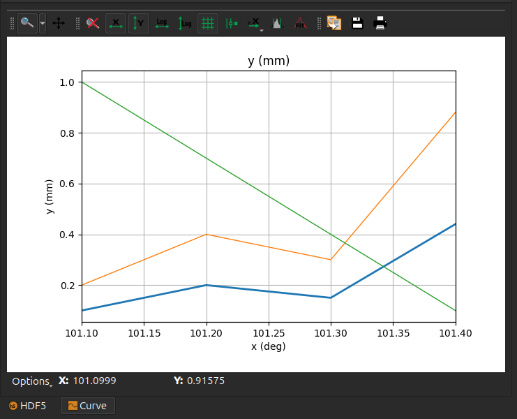
The simplest NXdata example would be a 1D signal to be plotted as a curve.
import h5py
import numpy

with h5py.File("myfile.h5", "w") as h5file:
    # It is mandatory to have at least one NXentry
    # https://manual.nexusformat.org/classes/base_classes/NXentry.html#nxentry
    entry = h5file.create_group("entry")
    entry.attrs["NX_class"] = "NXentry"

    nxdata = entry.create_group("my_curve")
    nxdata.attrs["NX_class"] = "NXdata"
    nxdata.attrs["signal"] = "y"
    ds = nxdata.create_dataset("y", data=numpy.array([0.1, 0.2, 0.15, 0.44]))

    # Add units (optional)
    ds.attrs["units"] = "mm"

    # Add an axis (optional)
    nxdata.attrs["axes"] = ["x"]
    ds = nxdata.create_dataset("x", data=numpy.array([101.1, 101.2, 101.3, 101.4]))
    ds.attrs["units"] = "deg"

    # Add additional curves with auxiliary signals (optional)
    nxdata.create_dataset("y2", data=numpy.array([0.2, 0.4, 0.3, 0.88]))
    nxdata.create_dataset("y3", data=numpy.array([1, 0.7, 0.4, 0.1]))
    nxdata.attrs["auxiliary_signals"] = ["y2", "y3"]
This will give the following plot in silx view:
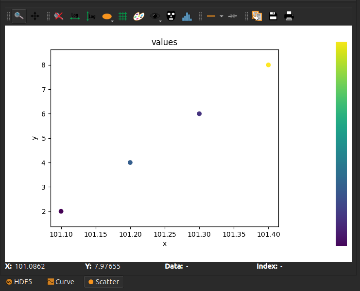
A 2D scatter plot#
A scatter plot is the only case for which we can have more axes than there are signal dimensions. The signal is 1D, and there can be any number of axes with the same number of values as the signal.
Silx supports 2D and 3D scatters.
To generate a 2D scatter plot:
import h5py
import numpy

with h5py.File("myfile.h5", "w") as h5file:
    entry = h5file.create_group("entry")
    entry.attrs["NX_class"] = "NXentry"

    nxdata = entry.create_group("my_scatter")
    nxdata.attrs["NX_class"] = "NXdata"
    nxdata.attrs["signal"] = "values"
    nxdata.attrs["axes"] = ["x", "y"]
    nxdata.create_dataset("values", data=numpy.array([0.1, 0.2, 0.15, 0.44]))
    nxdata.create_dataset("x", data=numpy.array([101.1, 101.2, 101.3, 101.4]))
    nxdata.create_dataset("y", data=numpy.array([2, 4, 6, 8]))
Again, in silx view:
A 3D scatter plot#
A 3D scatter plot can be generated likewise
import h5py
import numpy

with h5py.File("myfile.h5", "w") as h5file:
    entry = h5file.create_group("entry")
    entry.attrs["NX_class"] = "NXentry"

    nxdata = entry.create_group("my_3D_scatter")
    nxdata.attrs["NX_class"] = "NXdata"
    nxdata.attrs["signal"] = "values"
    nxdata.attrs["axes"] = ["x", "y", "z"]
    nxdata.create_dataset("values", data=numpy.array([0.1, 0.2, 0.15, 0.44]))
    nxdata.create_dataset("x", data=numpy.array([101.1, 101.2, 101.3, 101.4]))
    nxdata.create_dataset("y", data=numpy.array([2, 4, 6, 8]))
    nxdata.create_dataset("z", data=numpy.array([-10, -8, -6, -4]))
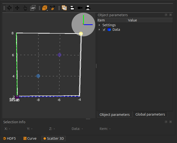
Note
When producing the 3D scatter plot, silx view will scale the markers according to the first auxiliary signal.
nxdata.create_dataset("sizes", data=numpy.array([2, 4, 4, 2]))
nxdata.attrs["auxiliary_signals"] = ["sizes"]
If there is no auxiliary signal, all markers will have the same size.
A stack of images#
In case of a stack, the first axis corresponds to stack indices and may not be represented by a dataset.
In this case, we use . as a placeholder in axes for this dimension:
import h5py
import numpy

with h5py.File("myfile.h5", "w") as h5file:
    entry = h5file.create_group("entry")
    entry.attrs["NX_class"] = "NXentry"

    nxdata = entry.create_group("image")
    nxdata.attrs["NX_class"] = "NXdata"
    nxdata.attrs["signal"] = "frames"
    nxdata.attrs["axes"] = [".", "y", "x"]
    # 2 frames of size 3 rows x 4 columns
    signal = nxdata.create_dataset(
        "frames",
        data=numpy.array(
            [
                [[1.0, 1.1, 1.2, 1.3], [1.4, 1.5, 1.6, 1.7], [1.8, 1.9, 2.0, 2.1]],
                [[8.0, 8.1, 8.2, 8.3], [8.4, 8.5, 8.6, 8.7], [8.8, 8.9, 9.0, 9.1]],
            ]
        ),
    )
    x = nxdata.create_dataset("x", data=numpy.array([0.1, 0.2, 0.3, 0.4]))
    x.attrs["units"] = "mm"
    y = nxdata.create_dataset("y", data=numpy.array([2, 4, 6]))
    y.attrs["units"] = "s"
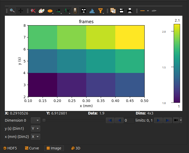
Note
If the image axes have the same units or both have no units, the image aspect ratio will kept.
In the example above, the two axes x and y have different units so that the image aspect ratio is not conserved.