Tutorial for fluorescence reconstruction
Note
in order to run this tutorial the installation of freeart (and tomogui) is mandatory.
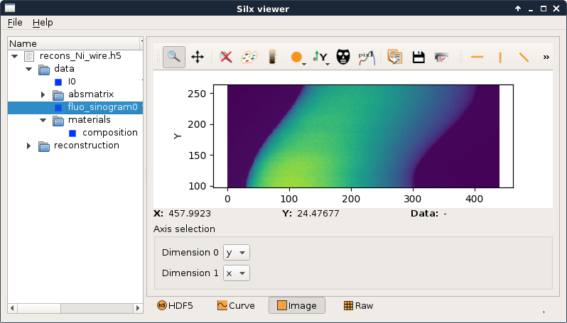
The tutorial is using the recons_Ni_wire.h5 file located in tomogui/example.
This file contains all the requested data for reconstructing a fluorescence sinogram.
- Ni fluorescence sinogram (h5 path: /data/fluo_sinogram0) obtain from pymca.
- I0 sinogram (h5 path: /data/I0)
- It sinogram (h5 path: /data/absmatrix/absm25)
It also contains the reconstruction configuration for running the fluorescence reconstruction from tomogui and freeart (h5 path: /reconstruction).
Note
you can browse the .h5 file using the silx view command for example (silx is a mandatory dependancy of tomogui).
silx view example/recons_Ni_wire.h5
goal
The goal of this tutorial is to run a ** Fluorescence ART reconstruction** (from the Ni fluorescence sinogram). This type of reconstruction take into account:
- the absorption of the incoming beam (aka absorption).
- the absorption of the outgoing beam (aka self attenuation)
For this we need:
- an absorption matrix. obtained from \({I_0}\) and \({I_t}\) sinograms.
- fluorescence sinogram(s) (Ni sinogram here)
- self attenuation matrices (one per fluorescence sinogram. Here one)
- information about the acquisition setup
All requested information are on the given file. We will explain latter how to obtain the self attenuation matrix. We now only need to get a few more information about the acquisition setup.
To have more information about the algorithm see the freeart fluorescence documentation
acquisition setup
We are considering the following setup for the acquisition
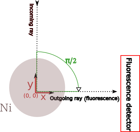
- the diameter of the wire is 25 \({\mu}m\)
- steps of 0.1 \({\mu}m\)
- \({E_0}\) (Ni -KL3) is 29.6 keV
- \({E_F}\) is 7.478 keV
- the detector is positioned at 90 degree from the sample. far away at 1000 cm from the sample center (simplification of the set up)
- full acquisition (360 degree)
Note
the example contains all the requested dataset. But for now the project files are storing path in absolute. So you can’t load directly the given example file. This should be fixed in the next release.
Now we can start the hand on by creating a new project file.
you can create a new project from using:
tomogui project
Note
Later you will be able to load back your project using the command:
tomogui project recons_Ni_wire.h5
definition of the reconstruction
The first thing to do is to define the type of reconstruction we want to run. This tutorial will focus on a fluorescence reconstruction so we will pick the Fluorescence (freeart) option. And we will go through all the tabs existing.
data source
The data source tab is used to define the sinogram to be reconstructed.
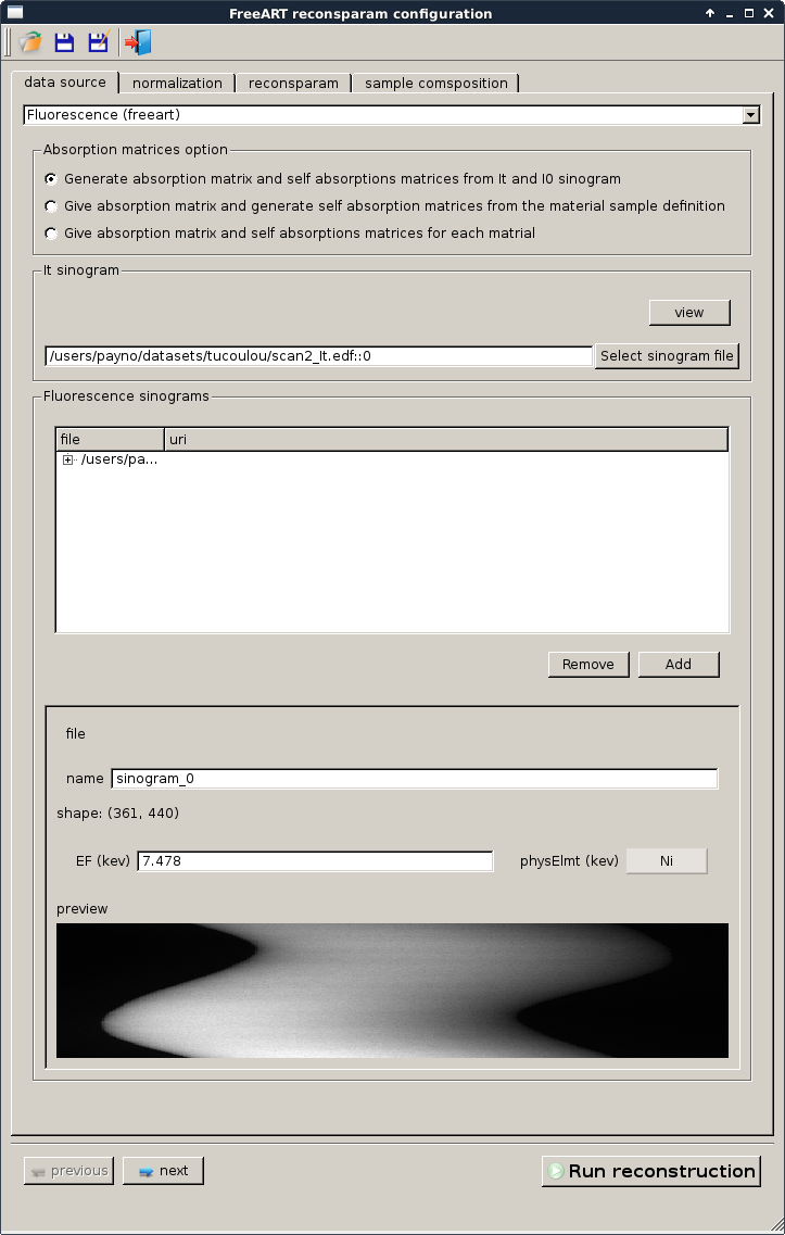
absorption matrix and It sinogram
As explained previously the first thing we need is an absorption matrix. For this we have two options:
- give It and I0 and generate the absorption matrix from an absorption reconstruction (option “Generate absorption matrix and self attenuations matrices from \(I_t\) and \(I_0\) sinogram”)
- give directly the absorption matrix if you have it (options “Give absorption matrix and generate self attenuation matrices from the material sample definition” and “Give absorption matrix and self attenuations matrices for each matrial”)
In our case we want to create the absorption matrix from \(I_t\) and \(I_0\) which is the ‘simplest’ way to obtain the absorption matrix.
Here we will take time to show you how to select a sinogram. The image selection dialog is the same for all sinogram and matrix selection.
Click on select sinogram file and browse to the h5 path /data/absmatrix/absm25.
sinogram and matrix selection
On the \({I_t}\) group click on select sinogram file. The following dialog should appear
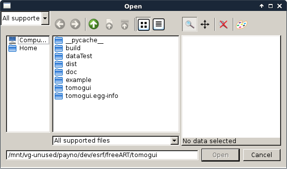
Then using this silx Dialog you can select a specific image. It allows picking from a .h5 file and from a single or multi frame edf file. If the file contains multiple image you can browse it until reaching the targetted image.
Fluorescence sinogram
The fluorescence sinogram is already registred. To add one more fluorescence sinogram we can activate the add button. Then we select a file (and an adress for h5 file) as explained in sinogram and matrix selection
Now for each fluorescence sinogram (only one in our case) we:
- can define a name. A default name is proposed.
- have to give \(E_F\) and the element if we didn’t pick the Give absorption matrix and self attenuations matrices for each matrial option
- have to give the path to the self attenuation matrix if we activate the Give absorption matrix and self attenuations matrices for each matrial option
This operation has to be done for all fluorescence sinogram in order to have the correct self absortion matrices.
Note
If you don’t have \({I_t}\) and \({I_0}\) you can create absorption matrix from the definition of materials with their densities and the energy of the beam. See tomogui creator for more information.
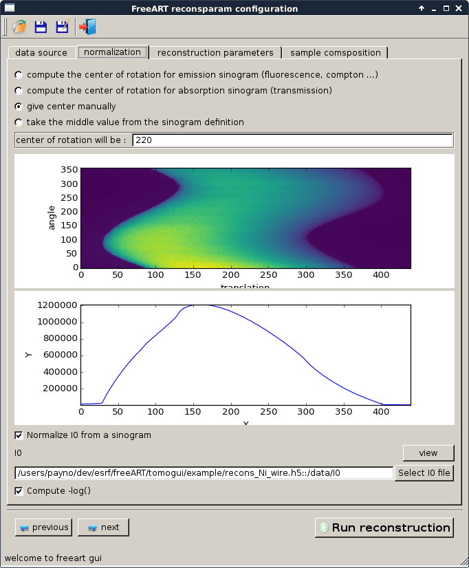
normalization
The normalization tab is used to set three main information:
- the center of rotation that can be given manually or guess by the software. For this example we will pick 215. For now it only deal with integer values.
- information about \({I_0}\). Each sinogram reconstructed will be normalized from this.
- compute -log option. This is used for the freeart transmission reconstruction only. Freeart needs \(-log(\frac{I_t}{I_0})\) to un the ART transmission reconstruction. By default you should give the algorithm \(I_t\) and \(I_0\). In this case the -log option should be activated. But in some cases user have already \(-log(\frac{I_t}{I_0})\) so they should uncheck this option and give \(I_0\) to a numerical value of 1.
Note
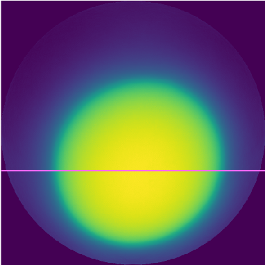
We highly recommended to normalize from a sinogram which will take into account the evolution of the energy of the beam through projection. Here is an example of a reconstruction using a single value for \(I_0\) (in the left) and using the true \(I_0\) sinogram in the right.
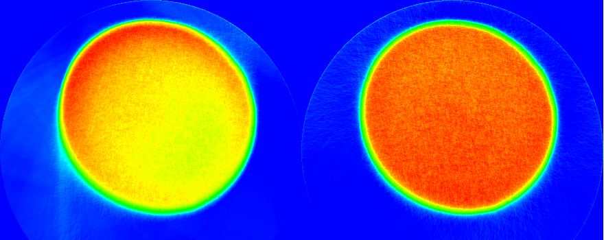
The aureole come from a bad definition center of rotation. On this example we picked 220 instead of 215
reconstruction parameters
This tab contains the parameters used by the ART algorithm. It has been tuned according to the knoledge we had of the acquisition setup
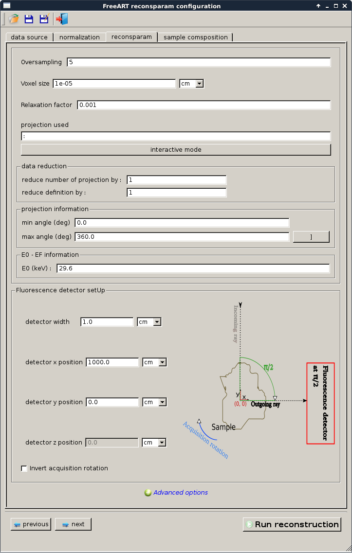
- oversampling will impact the quality of your reconstruction. We can see it as the number of sample point per pixel that will be computed to estimate the reconstruction and absorptions.
- voxel size This information is very important. As absorption and self attenuation are normalized (\(g.cm^{-2}\)) the voxel size will impact directly the effect of the incoming and outgoing beams. So if the effect of the absorption and the self attenuations is underestimate or overestimate it might be the origin.
- relaxation factor is used by the ART algorithms. By default a value is proposed which is supposed to be optimal value. A large modification of it can bring to bad reconstruction (having large blur) or having only a fiew pixel reconstructed.
- projections used as this is an ART reconstruction we can select the projection to take into account and ‘skip’ some. You can use the interactive mode to select them.
- data reduction is used for large sinogram and/or fast reconstruction we may want to take only a part of the projection and the pixel of the detector.
- projection information is needed to know the angle of the first and the last projections of the sinograms. If your acquisition is an half acquisition (180 degree) and you don’t informe the ART reconstruction of it, it will generate bad result.
- E0 is necessary to generate correct self attenuation we need to compute \({\mu}_{E_0}\) and \({\mu}_{E_F}\) and to do so we need information about \({E_0}\) and \({E_F}\).
- detector set up has to be know to compute correct rays path we need to know about the direction of those. At least the relative position is needed. A correct position is needed to compute the real solid angle for each pixel. You can force the solid angle calculation to be set to 1 in the advanced options.
sample composition
To compute the self attenuation of each pixel as explained in reconstruction parameters we need to know \({E_F}\) and \({E_0}\) but also the material contained per each pixel in order to compute the correct \({\mu}_{E_0}\) and \({\mu}_{E_F}\) per pixel (using the fisx library.). So this is why we need the sample composition for the options “Generate absorption matrix and self attenuations matrices from \({I_t}\) and \({I_0}\) sinogram” and “Give absorption matrix and generate self attenuation matrices from the material sample definition”
On this example the sample composition is already define but to create a new material you can simply use the add material button then the following interface appears fron which you can define the material. The sample composition definition can be made during the definition of the reconstruction or it will be triggered by the software before the Fluorescence sinogram reconstruction.
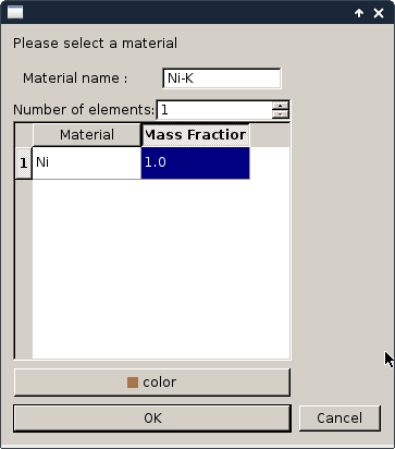
Once your material is defined you can draw on the image the location of each material. On this particular example the sample is only composed of one material. But the freeart library is able to deal with several.
Warning
One pixel can have at least one material definition. It will take the lower one on the list.
Note
You need to have a ‘background’ to know dimension of the sample and get an overview of the shape. Usually it is obtain fron the absorption matrix. If you wan’t to define it before you can try the try to guess background button which will make a FBP reconstruction from It. But this is not guaranty to work in all cases. The other option in the case you already have a view of you sample in an .edf or .h5 file is to load it in background manually using the ‘change background image’
Now that your project is fully defined you can start the reconstruction of the fluorescence sinogram. using the reconstruction button.
Note
If you saved your project you can open it directly using:
tomogui project myProjectFile.h5
to access the definition of the reconstruction interface or using
tomogui recons myProject.h5
to access the reconstruction interface or using
reconstruction
First the software detects that he doesn’t have absorption matrices yet. So he need to reconstruct it using the ART transmission algorithm.
Absorption matrix reconstruction
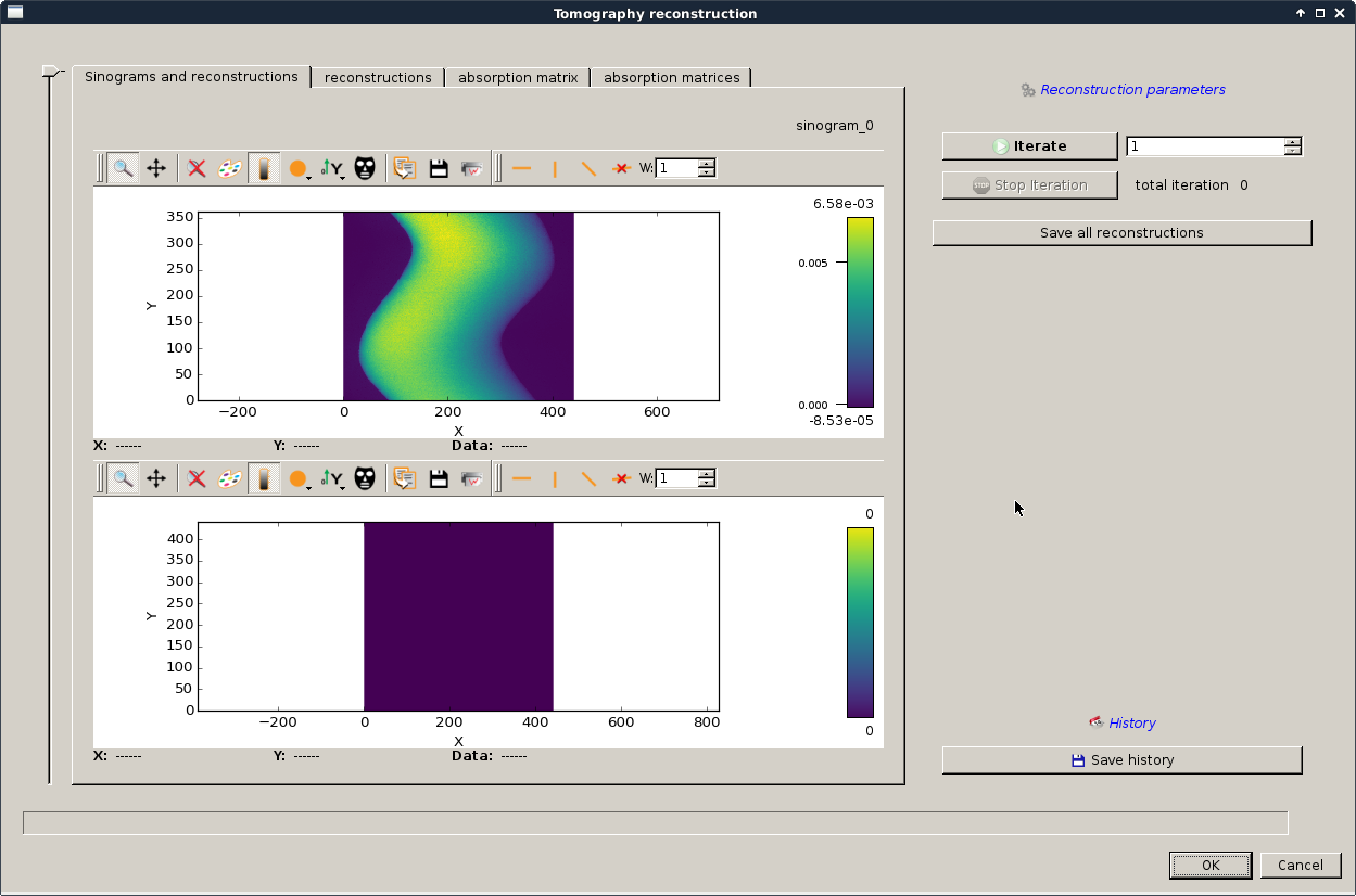
The following dialog should appear in order to reconstruct the absorption matrix from \({I_t}\) and \({I_0}\):
You can now run a few iteration on the ART transmission reconstruction using the iterate button. Iterate until you obtain something like looking like your sample:
Note
if your number of iteration and/or your relaxation factor is/are underestimated you might end up with something like this:
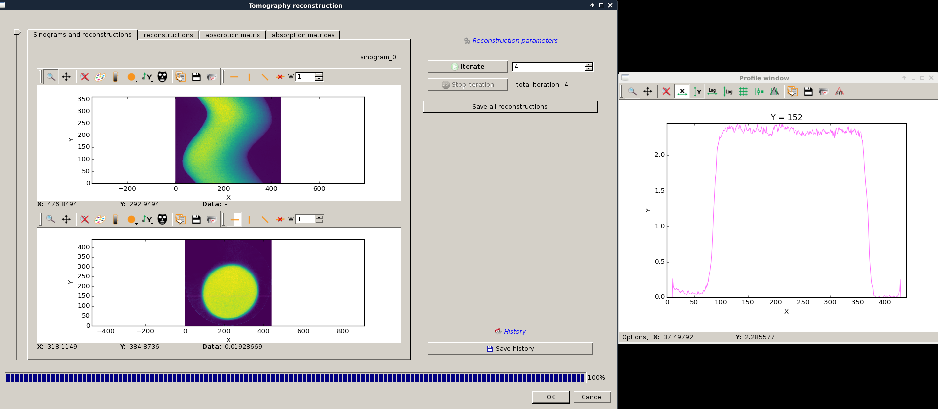
Here is the profile of the reconstruction:
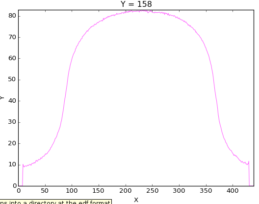
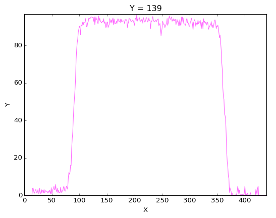
And as you can notice by the blur effect the ART algorithm hasn’t converge. So this need probably more iteration or your relaxation factor is way to small. We can compare it with the profile obtained on the valid reconstruction
When you have a reconstruction which seems valid for you validate it by clicking the ok button.
Note
if you had set an absorption matrix in tomogui instead of \(I_t\) and \(I_0\) sinograms, this part would have been skipped.
Sample composition definition
Here you will be asked to validate the composition of the sample. The necessity of it has been discussed previously. If you haven’t done it please set it as explained in sample composition.
Note
if you had set the self attenuation matrix in tomogui instead of defining the element of the sinogram and \(E_F\) this part would have been skipped.
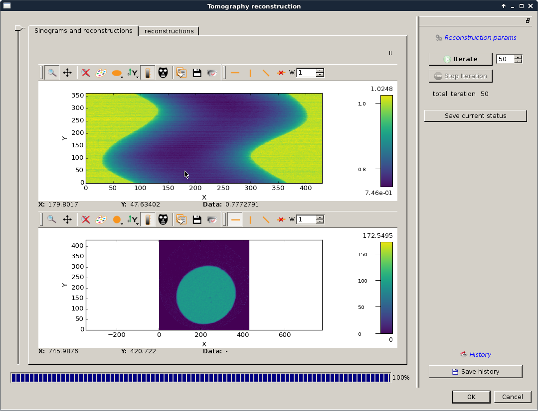
Fluorescence sinogram reconstruction
This is the last interface which should allow you to run reconstruction and browse on the data base used to run this reconstruction.
I hope tab names are self-describing.
The slider on the left will allow you to browse through the different fluorescence sinograms. In this case we have only one.
Now you have to launch iteration(s) to run the reconstruction.
After a few iteration you should see the something close to the following reconstruction.
Note
having a look at the profile is a good indication to know if you had enough iterations.
Warning
this is an ART algorithm so it might need some time/iteration to converge to a satisfying solution.
Once you are satisfy about your reconstruction(s) you can save them
- using directly the silx’s plot action.
- using the save all reconstruction which will ask for a folder and save all under a predefined name.
Now you should be able to run fluorescence reconstruction from your own datasets.
Note
for now the reconstructed absorption matrix and self attenuation matrix are not saved automatically on the configuration. So if you plain to launch several time the reconstruction it might be interesting to save those matrices and set a new project using those.