Fit tools

Using leastsq()

Running an iterative fit with leastsq() involves the following steps:

• designing a fit model function that has the signature f(x, ...), where x is an array of values of the independent variable and all remaining parameters are the parameters to be fitted
• defining the sequence of initial values for all parameters to be fitted. You can usually start with [1., 1., ...] if you don’t know a better estimate. The algorithm is robust enough to converge to a solution most of the time.
• setting constraints (optional)

Data required to perform a fit is:

• an array of x values (abscissa, independent variable)
• an array of y data points
• the sigma array of uncertainties associated to each data point. This is optional, by default each data point gets assigned a weight of 1.

Default (unweighted) fit

Let’s demonstrate this process in a short example, using synthetic data. We generate an array of synthetic data using a polynomial function of degree 4, and try to use leastsq() to find back the functions parameters.

import numpy
from silx.math.fit import leastsq

# create some synthetic polynomial data
x = numpy.arange(1000)
y = 2.4 * x**4 - 10. * x**3 + 15.2 * x**2 - 24.6 * x + 150.

# define our fit function: a generic polynomial of degree 4
def poly4(x, a, b, c, d, e):
    return a * x**4 + b * x**3 + c * x**2 + d * x + e

# The fit is an iterative process that requires an initial
# estimation of the parameters. Let's just use 1s.
initial_parameters = numpy.array([1., 1., 1., 1., 1.])

# Run fit
fitresult = leastsq(model=poly4,
                    xdata=x,
                    ydata=y,
                    p0=initial_parameters,
                    full_output=True)

# leastsq with full_output=True returns 3 objets
optimal_parameters, covariance, infodict = fitresult
# the first object is an array with the fitted parameters
a, b, c, d, e = optimal_parameters

print("Fit took %d iterations" % infodict["niter"])
print("Reduced chi-square: %f" % infodict["reduced_chisq"])
print("Theoretical parameters:\n\t" +
      "a=2.4, b=-10, c=15.2, d=-24.6, e=150")
print("Optimal parameters for y2 fitting:\n\t" +
      "a=%f, b=%f, c=%f, d=%f, e=%f" % (a, b, c, d, e))

The output of this program is:

Fit took 35 iterations
Reduced chi-square: 682592.670690
Theoretical parameters:
    a=2.4, b=-10, c=15.2, d=-24.6, e=150
Optimal parameters for y fitting:
    a=2.400000, b=-9.999665, c=14.970422, d=31.683448, e=-3216.131136

Note

The exact results may vary depending on your Python version.

We can see that this fit result is poor. In particular, parameters d and e are very poorly fitted.

This is due to the fact that data points with large values have a stronger influence in the fit process. In our examples, as x increases, y increases fast. The influence of the weighting, and how to solve this issue is explained in more details in the next section.

In the meantime, if you simply limit the x range, to deal with smaller y values, you can notice that the fit result becomes perfect.

In our example, replacing x with:

x = numpy.arange(100)

produces the following result:

Fit took 9 iterations
Reduced chi-square: 0.000000
Theoretical parameters:
    a=2.4, b=-10, c=15.2, d=-24.6, e=150
Optimal parameters for y fitting:
    a=2.400000, b=-10.000000, c=15.200000, d=-24.600000, e=150.000000

Weighted fit

Since the fitting algorithm minimizes the sum of squared differences between input and evaluated data, points with higher y value had a greater weight in the fitting process. A solution to this problem, if we want to improve our fit, is to define uncertainties for the data. The larger the uncertainty on a data sample, the smaller its weight will be in the least-square problem.

It is important to set the uncertainties correctly, or you risk favoring either the lower values or the higher values in your data.

The common approach in counting experiments is to use the square-root of the data values as the uncertainty value (assuming a Poissonian law). Let’s apply it to our previous example:

sigma = numpy.sqrt(y)

# Fit y
fitresult = leastsq(model=poly4,
                    xdata=x,
                    ydata=y,
                    sigma=sigma,
                    p0=initial_parameters,
                    full_output=True)

This results in a great improvement:

Weighted fit took 6 iterations
Reduced chi-square: 0.000000
Theoretical parameters:
    a=2.4, b=-10, c=15.2, d=-24.6, e=150
Optimal parameters for y fitting:
    a=2.400000, b=-10.000000, c=15.200000, d=-24.600000, e=150.000000

The resulting fit is perfect. The fit converged even faster than when we limited x range to 0 – 100.

To use a real world example, when fitting x-ray fluorescence spectroscopy data, this common approach means that we consider the variance of each channel to be the number of counts in that channel. That corresponds to assuming a normal distribution. The true distribution being a Poisson distribution, the Gaussian distribution is a good approximation for channels with high number of counts, but the approximation is not valid when the number of counts in a channel is small.

Therefore, in spectra where the overall statistics is very low, a weighted fit can lead the fitting process to fit the background considering the peaks as outliers, because the fit will consider a channel with 1 count 100 times more relevant than a channel with 100 counts.

Constrained fit

But let’s revert back to our unweighted fit, to experiment with different approaches to improving the fit.

The leastsq() functions provides a way to set constraints on parameters. You can for instance assert that a given parameter must remain equal to it’s initial value, or define an acceptable range for it to vary, or decide that a parameter must be equal to another parameter multiplied by a certain factor. This is very useful in cases in which you have enough knowledge to make reasonable assumptions on some parameters.

In our case, we will set constraints on d and e. We will quote d to stay in the range between -25 and -24, and fix e to 150.

Replace the call to leastsq() by following lines:

# Define constraints
cons = [[0, 0, 0],          # a: no constraint
        [0, 0, 0],          # b: no constraint
        [0, 0, 0],          # c: no constraint
        [2, -25., -23.],    # -25 < d < -24
        [3, 0, 0]]          # e is fixed to initial value
fitresult = leastsq(poly4, x, y,
                    # initial values must be consistent with constraints
                    p0=[1., 1., 1., -24., 150.],
                    constraints=cons,
                    full_output=True)

The output of this program is:

Constrained fit took 100 iterations
Reduced chi-square: 3.749280
Theoretical parameters:
    a=2.4, b=-10, c=15.2, d=-24.6, e=150
Optimal parameters for y fitting:
    a=2.400000, b=-9.999999, c=15.199648, d=-24.533014, e=150.000000

The chi-square value is much improved and the results are much better, at the cost of more iterations.

Using FitManager

A FitManager is a tool that provides a way of handling fit functions, associating estimation functions to estimate the initial parameters, modify the configuration parameters for the fit (enabling or disabling weights...) or for the estimation function, and choosing a background model.

It provides an abstraction layer on top of leastsq().

Weighted polynomial fit

The following program accomplishes the same weighted fit of a polynomial as in the previous tutorial (Weighted fit)

import numpy
from silx.math.fit.fitmanager import FitManager

# Create synthetic data with a sum of gaussian functions
x = numpy.arange(1000).astype(numpy.float)
y = 2.4 * x**4 - 10. * x**3 + 15.2 * x**2 - 24.6 * x + 150.

# define our fit function: a generic polynomial of degree 4
def poly4(x, a, b, c, d, e):
    return a * x**4 + b * x**3 + c * x**2 + d * x + e

# define an estimation function to that returns initial parameters
# and constraints
def esti(x, y):
    p0 = numpy.array([1., 1., 1., 1., 1.])
    cons = numpy.zeros(shape=(5, 3))
    return p0, cons

# Fitting
fit = FitManager()
fit.setdata(x=x, y=y)

fit.addtheory("polynomial",
              function=poly4,
              # any list of 5 parameter names would be OK
              parameters=["A", "B", "C", "D", "E"],
              estimate=esti)
fit.settheory('polynomial')
fit.configure(WeightFlag=True)
fit.estimate()
fit.runfit()

print("\n\nFit took %d iterations" % fit.niter)
print("Reduced chi-square: %f" % fit.chisq)
print("Theoretical parameters:\n\t" +
      "a=2.4, b=-10, c=15.2, d=-24.6, e=150")
a, b, c, d, e = (param['fitresult'] for param in fit.fit_results)
print("Optimal parameters for y2 fitting:\n\t" +
      "a=%f, b=%f, c=%f, d=%f, e=%f" % (a, b, c, d, e))

The result is the same as in our weighted leastsq() example, as expected:

Fit took 6 iterations
Reduced chi-square: 0.000000
Theoretical parameters:
    a=2.4, b=-10, c=15.2, d=-24.6, e=150
Optimal parameters for y2 fitting:
    a=2.400000, b=-10.000000, c=15.200000, d=-24.600000, e=150.000000

Fitting gaussians

The FitManager object is especially useful for fitting multi-peak gaussian-shaped spectra. The silx module silx.math.fit.fittheories provides fit functions and their associated estimation functions that are specifically designed for this purpose.

These fit functions can handle variable number of parameters defining a variable number of peaks, and the estimation functions use a peak detection algorithm to determine how many initial parameters must be returned.

For the sake of the example, let’s test the multi-peak fitting on synthetic data, generated using another silx module: silx.math.fit.functions.

import numpy
from silx.math.fit.functions import sum_gauss
from silx.math.fit import fittheories
from silx.math.fit.fitmanager import FitManager

# Create synthetic data with a sum of gaussian functions
x = numpy.arange(1000).astype(numpy.float)

# height, center x, fwhm
p = [1000, 100., 250,     # 1st peak
     255, 690., 45,       # 2nd peak
     1500, 800.5, 95]     # 3rd peak

y = sum_gauss(x, *p)

# Fitting
fit = FitManager()
fit.setdata(x=x, y=y)
fit.loadtheories(fittheories)
fit.settheory('Gaussians')
fit.estimate()
fit.runfit()

print("Searched parameters = %s" % p)
print("Obtained parameters : ")
dummy_list = []
for param in fit.fit_results:
    print(param['name'], ' = ', param['fitresult'])
    dummy_list.append(param['fitresult'])
print("chisq = ", fit.chisq)

And the result of this program is:

Searched parameters = [1000, 100.0, 250, 255, 690.0, 45, 1500, 800.5, 95]
Obtained parameters :
('Height1', ' = ', 1000.0)
('Position1', ' = ', 100.0)
('FWHM1', ' = ', 250.0)
('Height2', ' = ', 255.0)
('Position2', ' = ', 690.0)
('FWHM2', ' = ', 44.999999999999993)
('Height3', ' = ', 1500.0)
('Position3', ' = ', 800.5)
('FWHM3', ' = ', 95.000000000000014)
('chisq = ', 0.0)

In addition to gaussians, we could have fitted several other similar type of functions: asymetric gaussian functions, lorentzian functions, pseudo-voigt functions or hypermet tailing functions.

The loadtheories() method can also be used to load user defined functions. Instead of a module, a path to a Python source file can be given as a parameter. This source file must adhere to certain conventions, as explained in the documentation of silx.math.fit.fittheories and silx.math.fit.fittheory.FitTheory.

Subtracting a background

FitManager provides a few standard background theories, for cases when a background signal is superimposed on the multi-peak spectrum.

For example, let’s add a linear background to our synthetic data, and see how FitManager handles the fitting.

In our previous example, redefine y as follows:

p = [1000, 100., 250,
     255, 690., 45,
     1500, 800.5, 95]
y = sum_gauss(x, *p)
# add a synthetic linear background
y += 0.13 * x + 100.

Before the line fit.estimate(), add the following line:

fit.setbackground('Linear')

The result becomes:

Searched parameters = [1000, 100.0, 250, 255, 690.0, 45, 1500, 800.5, 95]
Obtained parameters :
('Constant', ' = ', 100.00000000000001)
('Slope', ' = ', 0.12999999999999998)
('Height1', ' = ', 1000.0)
('Position1', ' = ', 100.0)
('FWHM1', ' = ', 249.99999999999997)
('Height2', ' = ', 255.00000000000003)
('Position2', ' = ', 690.0)
('FWHM2', ' = ', 44.999999999999993)
('Height3', ' = ', 1500.0)
('Position3', ' = ', 800.5)
('FWHM3', ' = ', 95.0)
('chisq = ', 3.1789004676997597e-27)

The available background theories are: Linear, Constant and Strip.

The strip background is a popular background model that can compute and subtract any background shape as long as its curvature is significantly lower than the peaks’ curvature. In other words, as long as the background signal is significantly smoother than the actual signal, it can be easily computed.

The main parameters required by the strip function are the strip width w and the number of iterations. At each iteration, if the contents of channel i, y(i), is above the average of the contents of the channels at w channels of distance, y(i-w) and y(i+w), y(i) is replaced by the average. At the end of the process we are left with something that resembles a spectrum in which the peaks have been “stripped”.

The following example illustrates the strip background removal process:

from silx.sx import plot
from silx.gui import qt
import numpy
from silx.math.fit.filters import strip
from silx.math.fit.functions import sum_gauss

x = numpy.arange(5000)
# (height1, center1, fwhm1, ...) 5 peaks
params1 = (50, 500, 100,
           20, 2000, 200,
           50, 2250, 100,
           40, 3000, 75,
           23, 4000, 150)
y0 = sum_gauss(x, *params1)

# random values between [-1;1]
noise = 2 * numpy.random.random(5000) - 1
# make it +- 5%
noise *= 0.05

# 2 gaussians with very large fwhm, as background signal
actual_bg = sum_gauss(x, 15, 3500, 3000, 5, 1000, 1500)

# Add 5% random noise to gaussians and add background
y = y0 * (1 + noise) + actual_bg

# compute strip background model
strip_bg = strip(y, w=5, niterations=5000)

# plot results
app = qt.QApplication([])
plot(x, y, x, actual_bg, x, strip_bg)
plot(x, y, x, (y - strip_bg))
app.exec_()

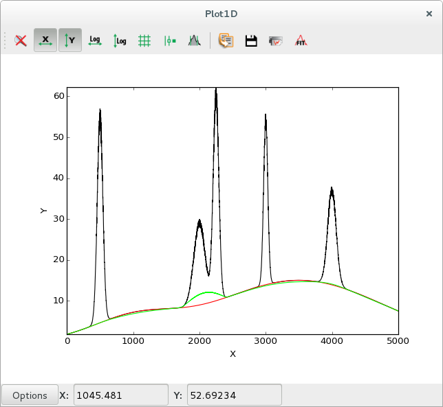	Data with background in black (y), actual background in red, computed strip background in green
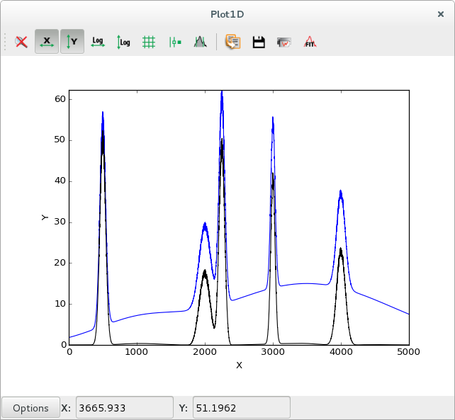	Data with background in blue, data after subtracting strip background in black

The strip also removes the statistical noise, so the computed strip background will be slightly lower than the actual background. This can be solved by performing a smoothing prior to the strip computation.

See the PyMca documentation for more information on the strip background.

To configure the strip background model of FitManager, use its configure() method to modify the following parameters:

• StripWidth: strip width parameter w, mentionned earlier
• StripNIterations: number of iterations
• StripThresholdFactor: if this parameter is left to its default value 1, the algorithm behaves as explained earlier: y(i) is compared to the average of y(i-1) and y(i+1). If this factor is set to another value f, y(i) is compared to the average multiplied by f.
• SmoothStrip: if this parameter is set to True, a smoothing is applied prior to the strip.

These parameters can be modified like this:

# ...
fit.settheory('Strip')
fit.configure(StripWidth=5,
              StripNIterations=5000,
              StripThresholdFactor=1.1,
              SmoothStrip=True)
# ...

Using a strip background has performance implications. You should try to keep the number of iterations as low as possible if you need to run batch fitting using this model. Increasing the strip width can help reducing the number of iterations, with the risk of underestimating the background signal.

Using FitWidget

Simple usage

The FitWidget is a graphical interface for FitManager.

import numpy
from silx.gui import qt
from silx.gui.fit import FitWidget
from silx.math.fit.functions import sum_gauss

x = numpy.arange(2000).astype(numpy.float)
constant_bg = 3.14

# gaussian parameters: height, position, fwhm
p = numpy.array([1000, 100., 30.0,
                 500, 300., 25.,
                 1700, 500., 35.,
                 750, 700., 30.0,
                 1234, 900., 29.5,
                 302, 1100., 30.5,
                 75, 1300., 75.])
y = sum_gauss(x, *p) + constant_bg

a = qt.QApplication([])

w = FitWidget()
w.setData(x=x, y=y)
w.show()

a.exec_()

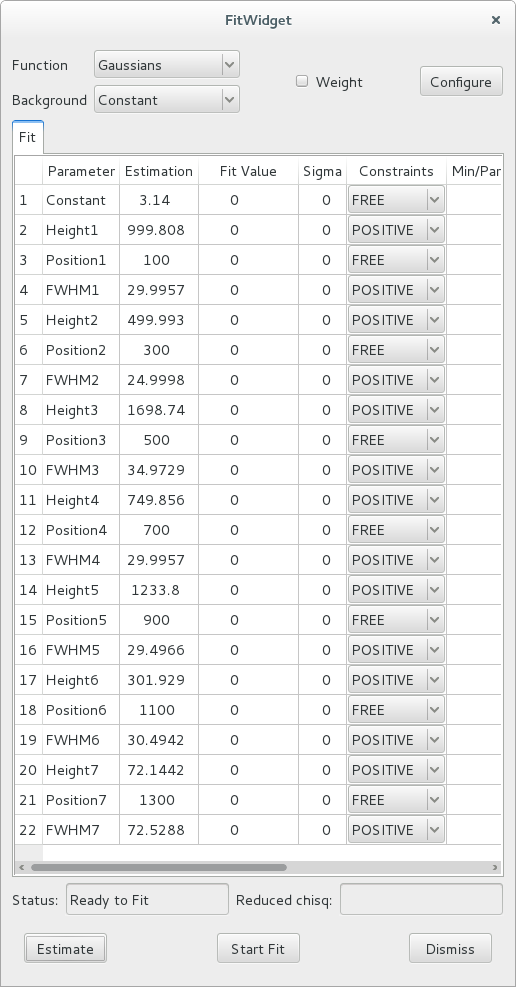
Executing this code opens the following widget.

The functions you can choose from are the standard gaussian-shaped functions from silx.math.fit.fittheories. At the top of the list, you will find the Add Function(s) option, that allows you to load your user defined fit theories from a .py source file.

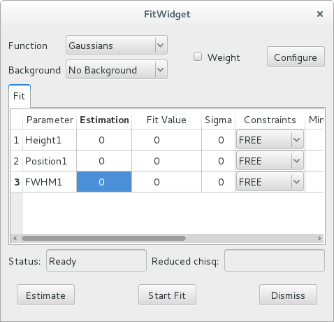
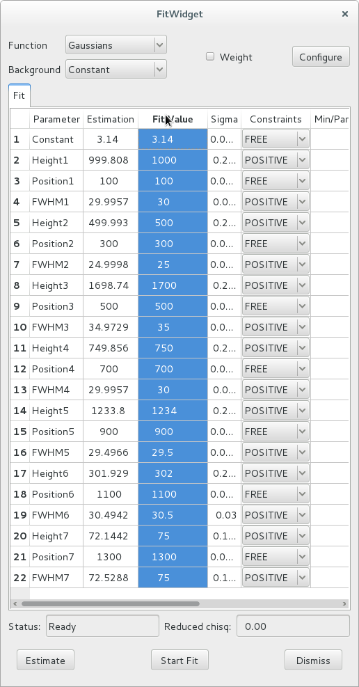
After selecting the Constant background model and clicking the Estimate button, the widget displays this:

The 7 peaks have been detected, and their parameters estimated. Also, the estimation function defined some constraints (positive height and positive full-width at half-maximum).

You can modify the values in the estimation column of the table, to use different initial parameters for the fit.

The individual constraints can be modified prior to fitting. It is also possible to modify the constraints globally by clicking the Configure button’ to open a configuration dialog. To get help on the meaning of the various parameters, hover the mouse on the corresponding check box or entry widget, to display a tooltip help message.

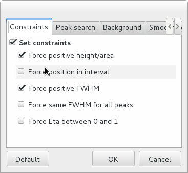
The other configuration tabs can be modified to change the peak search parameters and the strip background parameters prior to the estimation. After closing the configuration dialog, you must re-run the estimation by clicking the Estimate button.

After all configuration parameters and all constrants are set according to your preferences, you can click the Start Fit button. This runs the fit and displays the results in the Fit Value column of the table.

Customizing the functions

The FitWidget can be initialized with a non-standard FitManager, to customize the available functions.

from silx.gui import qt
from silx.math.fit import FitManager
from silx.gui.fit import FitWidget

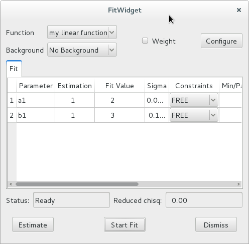
def linearfun(x, a, b):
    return a * x + b

# create synthetic data for the example
x = list(range(0, 100))
y = [linearfun(x_, 2.0, 3.0) for x_ in x]

# we need to create a custom fit manager and add our theory
myfitmngr = FitManager()
myfitmngr.setdata(x, y)
myfitmngr.addtheory("my linear function",
                    function=linearfun,
                    parameters=["a", "b"])

a = qt.QApplication([])

# our fit widget can now use our custom fit manager
fw = FitWidget(fitmngr=myfitmngr)
fw.show()

a.exec_()

In our previous example, we didn’t load a custom FitManager. Therefore, the fit widget automatically initialized a fit manager and loaded the custom gaussian functions.

This time, we initialized our own FitManager and loaded our own function, so only this function is presented as an option in the GUI.

Our custom function does not provide an associated estimation function, so the default estimation function of FitManager was used. This default estimation function returns an array of ones the same length as the list of parameter names, and set all constraints to FREE.