General introduction to sift.
silx.image.sift, a parallel version of SIFT algorithm
SIFT (Scale-Invariant Feature Transform) is an algorithm developed by David Lowe in 1999. It is a worldwide reference for image alignment and object recognition. The robustness of this method enables to detect features at different scales, angles and illumination of a scene. The implementation available in silx uses OpenCL, meaning that it can run on Graphics Processing Units and Central Processing Units as well. Interest points are detected in the image, then data structures called descriptors are built to be characteristic of the scene, so that two different images of the same scene have similar descriptors. They are robust to transformations like translation, rotation, rescaling and illumination change, which make SIFT interesting for image stitching. In the fist stage, descriptors are computed from the input images. Then, they are compared to determine the geometric transformation to apply in order to align the images. silx.image.sift can run on most graphic cards and CPU, making it usable on many setups. OpenCL processes are handled from Python with PyOpenCL, a module to access OpenCL parallel computation API.
Introduction
The European Synchrotron Radiation Facility (ESRF) beamline ID21 developed a full-field method for X-ray absorption near-edge spectroscopy (XANES). Since the flat field images are not acquired simultaneously with the sample transmission images, a realignment procedure has to be performed. Serial SIFT implementation used to take about 8 seconds per frame, and one stack can have up to 500 frames. It is a bottleneck in the global process, therefore a parallel version had to be implemented. silx.image.sift differs from existing parallel implementations of SIFT in the way that the whole process is done on the device, enabling crucial speed-ups.
Launching silx.image.sift
silx.image.sift is written in Python, and handles the OpenCL kernels with PyOpenCL. This enables a simple and efficient access to GPU resources. The project is installed as a Python library and can be imported in a script.
Before image alignment, points of interest (keypoints) have to be detected in each image. The whole process can be launched by several lines of code.
How to use it
silx.image.sift is installed as part of silx and requires PyOpenCL to be useable. It generates a library that can be imported, then used to compute a list of descriptors from an image. The image can be in RGB values, but all the process is done on grayscale values. One can specify the devicetype, either CPU or GPU.
This computes and shows the keypoints on the input image. One can also launch silx.image.sift interactively with iPython :
from silx.image import sift
import numpy
import scipy.misc
image_rgb = scipy.misc.imread("my_image.jpg")
sift_ocl = sift.SiftPlan(template=image_rgb, devicetype="GPU")
kp = sift_ocl.keypoints(image_rgb)
print(kp[-1])
silx.image.sift files
The Python sources are in the silx.image.sift module:
from silx.image import sift
print(sift.__file__)
The file plan.py corresponds to the keypoint extraction and handles the whole process: from kernel compilation to descriptors generation as numpy array. The OpenCL kernels are distributed as resources in the “openCL” folder; they are compiled on the fly. Several kernels have multiple implementations, depending the architecture to run on.
The file match.py does the matching between two lists of keypoints returned by plan.py.
The file alignment.py does the image alignment : it computes the keypoints from two images (plan.py), then uses the matching result (match.py) to find out the transformation aligning the second image on the first.
Each of those module contain a class which holds GPU contexts, memory and kernel. They are expensive to instantiate and should be re-used as much as possible.
Overall process
The different steps of SIFT are handled by plan.py. When launched, it automatically choose the best device to run on, unless a device is explicitly provided in the options. All the OpenCL kernels that can be compiled are built on the fly. Buffers are pre-allocated on the device, and all the steps are executed on rge device (GPU). At each octave (scale level), keypoints are returned to the CPU and the buffers are re-used.
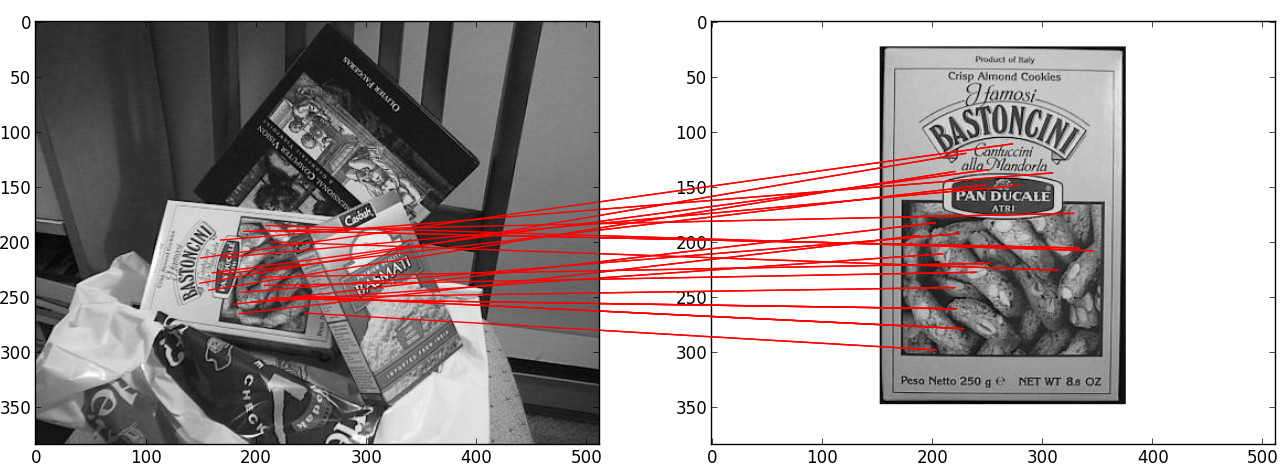
Once the keypoints are computed, the keypoints of two different images can be compared. This matching is done by match.py. It simply takes the descriptors of the two lists of keypoints, and compare them with a L1 distance. It returns a vector of matchings, i.e couples of similar keypoints.
For image alignment, alignment.py takes the matching vector between two images and determines the transformation to be done in order to align the second image on the first.
SIFT keypoints computation
The keypoints are detected in several steps according to Lowe’s paper :
- Keypoints detection: local extrema are detected in the scale-space \((x, y, s)\). Every pixel is compared to its neighborhood in the image itself, and in the previous/next scale factor images.
- Keypoints refinement: keypoints located on corners are discarded. Additionally, a second-order interpolation is done to improve the keypoints accuracy, modifying the coordinates \((x, y, s)\).
- Orientation assignment: a characteristic orientation is assigned to the keypoints \((x,y,s, \theta)\)
- Descriptor computation: a histogram of orientations is built around every keypoint, then concatenated in a 128-values vector. This vector is called SIFT descriptor, it is robust to rotation, illumination, translation and scaling.
The scale variation is simulated by blurring the image. A very blurred image represents a scene seen from a distance, for small details are not visible.
Unlike existing parallel versions of SIFT, the entire process is done on the device to avoid time-consuming transfers between CPU and GPU. This leads to several tricky parts like the use of atomic instructions, or writing different versions of the same kernel to adapt to every platform.
Keypoints detection
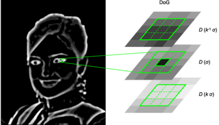
The image is increasingly blurred to imitate the scale variations. This is done by convolving with a gaussian kernel. Then, consecutive blurs are subtracted to get differences of gaussians (DoG). In these DoG, every pixel is tested. Let \((x,y)\) be the pixel position in the current (blurred) image, and \(s\) its scale (that is, the blur factor). The point \((x,y,s)\) is a local maximum in the scale-space if
- \(D(x-1, y, s) < D(x,y,s)\) and \(D(x,y,s) > D(x+1, y, s)\) (local maximum in \(x\))
- \(D(x, y-1, s) < D(x,y,s)\) and \(D(x,y,s) > D(x, y+1, s)\) (local maximum in \(y\))
- \(D(x, y, s -1) < D(x,y,s)\) and \(D(x,y,s) > D(x, y, s+1)\) (local maximum in \(s\))
For these steps, we highly benefit from the parallelism : every pixel is handled by a GPU thread. Besides, convolution is implemented in the direct space (without Fourier Transform) and is quite fast (50 times faster than the convolutions done by the C++ reference implementation).
Keypoints refinement
At this stage, many keypoints are not reliable. Low-contrast keypoints are discarded, and keypoints located on an edge are rejected as well. For keypoints located on an edge, principal curvature across the edge is much larger than the principal curvature along it. Finding these principal curvatures amounts to solving for the eigenvalues of the second-order Hessian matrix of the current DoG. The ratio of the eigenvalues \(r\) is compared to a threshold \(\dfrac{(r+1)^2}{r} < R\) with R defined by taking r=10.
To improve keypoints accuracy, the coordinates are interpolated with a second-order Taylor development.
\[D \left( \vec{x} + \vec{\delta_x} \right) \simeq D + \dfrac{\partial D}{\partial \vec{x}} \cdot \vec{\delta_x} + \dfrac{1}{2} \left( \vec{\delta_x} \right)^T \cdot \left( H \right) \cdot \vec{\delta_x} \qquad \text{with } H = \dfrac{\partial^2 D}{\partial \vec{x}^2}\]
Keypoints that were too far from a true (interpolated) extremum are rejected.
Orientation assignment
An orientation has to be assigned to each keypoint so that SIFT descriptors will be invariant to rotation. For each blurred version of the image, the gradient magnitude and orientation are computed. From the neighborhood of a keypoint, a histogram of orientations is built (36 bins, 1 bin per 10 degrees).
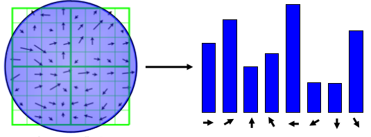
The maximum value of this histogram is the dominant orientation ; it is defined as the characteristic orientation of the keypoint. Additionally, every peak greater than 80% of the maximum generates a new keypoint with a different orientation.
The parallel implementation of this step is complex, and the performances strongly depend on the graphic card the program is running on. That is why there are different files for this kernel, adapted for different platforms. The file to compile is automatically determined in plan.py.
Descriptor computation
A histogram of orientations is built around every keypoint. The neighborhood is divided into 4 regions of 4 sub-regions of 4x4 pixels. In every sub-region, a 8-bin histogram is computed; then, all the histograms are concatenated in a 128-values descriptor. The histogram is weighted by the gradient magnitudes and the current scale factor, so that the descriptor is robust to rotation, illumination, translation and scaling. Here again, there are several files adapted to different platforms.
Performances
The aim of silx.image.sift is to fasten the SIFT keypoint extraction by running it on GPU. On big images with many keypoints, it enables a speed-up between 30 and 50 times. The following benchmark was done on an Intel Xeon E5-2667 (2.90GHz, 2x6 cores) CPU, and a NVidia Tesla K20m GPU.
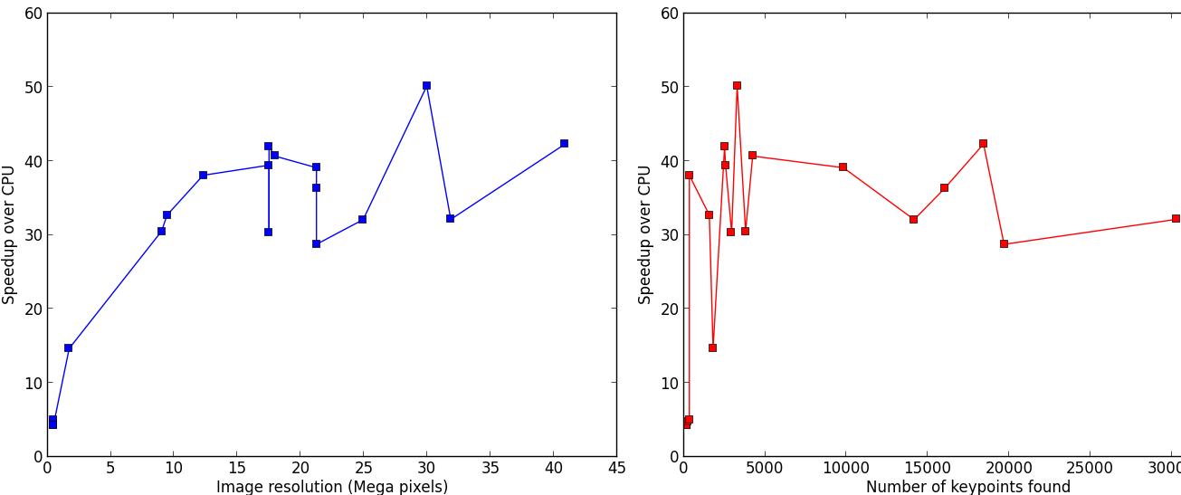
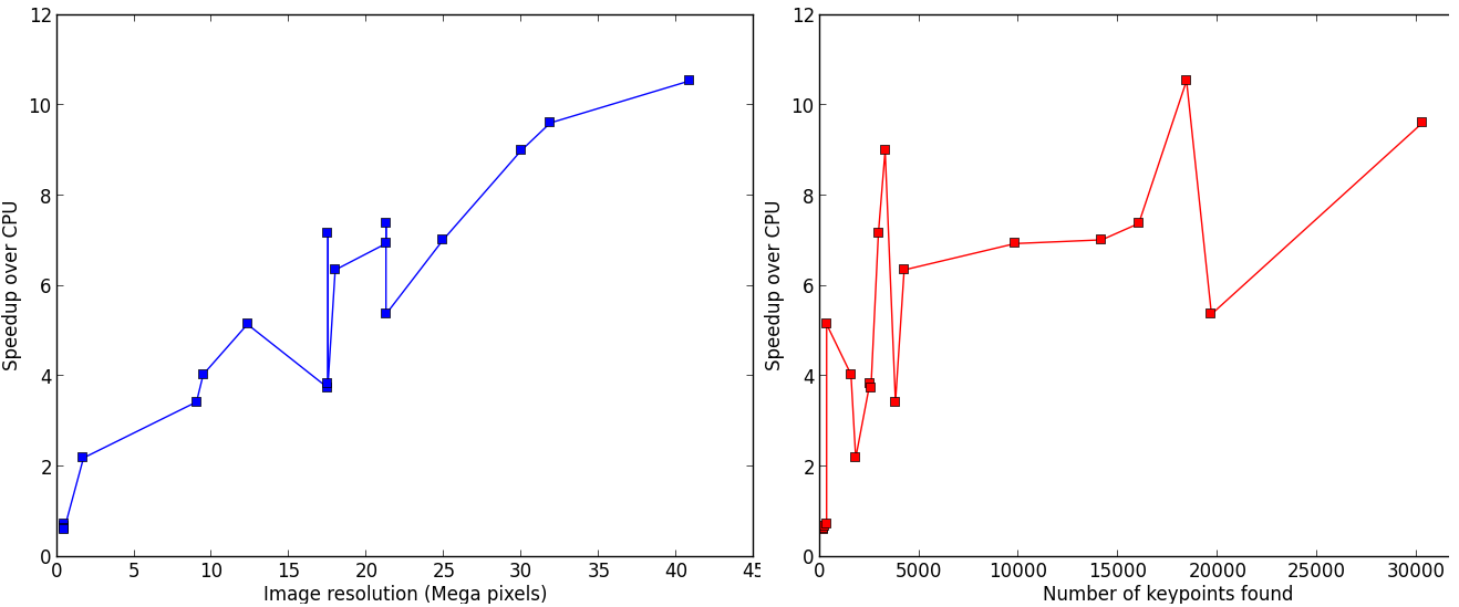
silx.image.sift can also be run on CPU, even running up to 10 times faster than the C++ implementation.
SIFT parameters
Command line parameters
When launched from the command line, silx.image.sift can handle several options like the device to run on and the number of pixels per keypoint. By default PIX_PER_KP is 10, meaning that we gess one keypoint will be found for every 10 pixels. This is for buffers allocation on the device, as the number of keypoints that will be found is unknown, and strongly depends of the type of image. 10 pixels per keypoint is a high estimation, even for images with many features like landscapes. For example, this 5.8 MPixels image gives about 2500 keypoints, which makes 2270 pixels per keypoints.
If you have big images with few features and the image does not fit on the GPU, you can increase PIX_PER_KP in the command line options in order to decrease the amount of memory required.
Advanced SIFT parameters
The file param.py contains SIFT default parameters, recommended by David Lowe in his paper or by the authors of the C++ version in ASIFT. You should not modify these values unless you know what you are doing. Some parameters require to understand several aspects of the algorithm, explained in Lowe’s original paper.
DoubleImSize (0 by default) is for the pre-blur factor of the image. At the beginning, the original image is blurred (prior-smoothing) to eliminate noise. The standard deviation of the gaussian filter is either 1.52 if DoubleImSize is 0, or 1.25 if DoubleImSize is 1. Setting this parameter to 1 decrease the prior-smoothing factor, the algorithm will certainly find more keypoints but less accurate.
InitSigma (1.6 by default) is the prior-smoothing factor. The original image is blurred by a gaussian filter which standard deviation is \(\sqrt{\text{InitSigma}^2 - c^2}\). with c == 0.5 if DoubleImSize == 0 or c == 1 otherwise. If the prior-smoothing factor is decreased, the algorithm will certainly find more keypoint, but they will be less accurate.
BorderDist (5 by default) is the minimal distance to borders: pixels that are less than BorderDist pixels from the border will be ignored for the processing. If features are likely to be near the borders, decreasing this parameter will enable to detect them.
Scales (3 by default) is the number of Difference of Gaussians (DoG) that will actually be used for keypoints detection. In the gaussian pyramid, Scales+3 blurs are made, from which Scales+2 DoGs are computed. The DoGs in the middle are used to detect keypoints in the scale-space. If Scales is 3, there will be 6 blurs and 5 DoGs in an octave, and 3 DoGs will be used for local extrema detection. Increasing Scales will make more blurred images in an octave, so SIFT can detect a few more strong keypoints. However, it will slow down the execution for few additional keypoints.
PeakThresh (255 * 0.04/3.0 by default) is the grayscale threshold for keypoints refinement. To discard low-contrast keypoints, every pixel which grayscale value is below this threshold can not become a keypoint. Decreasing this threshold will lead to a larger number of keypoints, which can be useful for detecting features in low-contrast areas.
EdgeThresh (0.06 by default) and EdgeThresh1 (0.08 by default) are the limit ratio of principal curvatures while testing if keypoints are located on an edge. Those points are not reliable for they are sensivite to noise. For such points, the principal curvature across the edge is much larger than the principal curvature along it. Finding these principal curvatures amounts to solving for the eigenvalues of the second-order Hessian matrix of the current DoG. The ratio of the eigenvalues \(r\) is compared to a threshold \(\dfrac{(r+1)^2}{r} < R\) with R defined by taking r=10, which gives \(\frac{(r+1)^2}{r} = 12.1\), and 1/12.1 = 0.08. In the first octave, the value 0.06 is taken instead of 0.08. Decreasing these values lead to a larger number of keypoints, but sensivite to noise because they are located on edges.
OriSigma (1.5 by default) is related to the radius of gaussian weighting in orientation assignment. In this stage, for a given keypoint, we look in a region of radius \(3 \times s \times \text{OriSigma}\) with \(s\) the scale of the current keypoint. Increasing it will not lead to increase the number of keypoints found; it will take a larger area into account while computing the orientation assignment. Thus, the descriptor will be characteristic of a larger neighbourhood.
MatchRatio (0.73 by default) is the threshold used for image alignment. Descriptors are compared with a \(L^1\)-distance. For a given descriptor, if the ratio between the closest-neighbor the second-closest-neighbor is below this threshold, then a matching is added to the list. Increasing this value leads to a larger number of matchings, certainly less accurate.
Region of Interest for image alignment
When processing the image matching, a region of interest (ROI) can be specified on the image. It is a binary image which can have any shape. For instance, if a sample is centered on the image, the user can select the center of the image before processing.
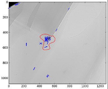
It both accelerates the processing and avoids to do match keypoints that are not on the sample.
References
- David G. Lowe, Distinctive image features from scale-invariant keypoints, International Journal of Computer Vision, vol. 60, no 2, 2004, p. 91–110 - “http://www.cs.ubc.ca/~lowe/papers/ijcv04.pdf“