Geometries in pyFAI

This notebook demonstrates the different orientations of axes in the geometry used by pyFAI.

Demonstration

The tutorial uses the Jypyter notebook.

import time
start_time = time.time()
%pylab nbagg

Populating the interactive namespace from numpy and matplotlib

import pyFAI
from pyFAI.gui import jupyter
from pyFAI.calibrant import get_calibrant

We will use a fake detector of 1000x1000 pixels of 100_µm each. The simulated beam has a wavelength of 0.1_nm and the calibrant chose is silver behenate which gives regularly spaced rings. The detector will originally be placed at 1_m from the sample.

wl = 1e-10
cal = get_calibrant("AgBh")
cal.wavelength=wl

detector = pyFAI.detectors.Detector(100e-6, 100e-6)
detector.max_shape=(1000,1000)

ai = pyFAI.AzimuthalIntegrator(dist=1, detector=detector)
ai.wavelength = wl

img = cal.fake_calibration_image(ai)
jupyter.display(img, label="Inital")

<IPython.core.display.Javascript object>

<matplotlib.axes._subplots.AxesSubplot at 0x7f20162011d0>

Translation orthogonal to the beam: poni1 and poni2

We will now set the first dimension (vertical) offset to the center of the detector: 100e-6 * 1000 / 2

p1 = 100e-6 * 1000 / 2
print("poni1:", p1)
ai.poni1 = p1
img = cal.fake_calibration_image(ai)
jupyter.display(img, label="set poni1")

poni1: 0.05

<IPython.core.display.Javascript object>

<matplotlib.axes._subplots.AxesSubplot at 0x7f201616e828>

Let’s do the same in the second dimensions: along the horizontal axis

p2 = 100e-6 * 1000 / 2
print("poni2:", p2)
ai.poni2 = p2
print(ai)
img = cal.fake_calibration_image(ai)
jupyter.display(img, label="set poni2")

poni2: 0.05
Detector Detector    Spline= None    PixelSize= 1.000e-04, 1.000e-04 m
Wavelength= 1.000000e-10m
SampleDetDist= 1.000000e+00m        PONI= 5.000000e-02, 5.000000e-02m       rot1=0.000000  rot2= 0.000000  rot3= 0.000000 rad
DirectBeamDist= 1000.000mm  Center: x=500.000, y=500.000 pix        Tilt=0.000 deg  tiltPlanRotation= 0.000 deg

<IPython.core.display.Javascript object>

<matplotlib.axes._subplots.AxesSubplot at 0x7f20161461d0>

The image is now properly centered. Let’s investigate the sample-detector distance dimension.

For this we need to describe a detector which has a third dimension which will be offseted in the third dimension by half a meter.

#define 3 plots
fig, ax = subplots(1, 3, figsize=(12,4))

import copy
ref_10 = cal.fake_calibration_image(ai, W=1e-4)
jupyter.display(ref_10, label="dist=1.0m", ax=ax[1])

ai05 = copy.copy(ai)
ai05.dist = 0.5
ref_05 = cal.fake_calibration_image(ai05, W=1e-4)
jupyter.display(ref_05, label="dist=0.5m", ax=ax[0])

ai15 = copy.copy(ai)
ai15.dist = 1.5
ref_15 = cal.fake_calibration_image(ai15, W=1e-4)
jupyter.display(ref_15, label="dist=1.5m", ax=ax[2])

<IPython.core.display.Javascript object>

<matplotlib.axes._subplots.AxesSubplot at 0x7f2016026358>

We test now if the sensot of the detector is not located at Z=0 in the detector referential but any arbitrary value:

class ShiftedDetector(pyFAI.detectors.Detector):
    IS_FLAT = False  # this detector is flat
    IS_CONTIGUOUS = True  # No gaps: all pixels are adjacents, speeds-up calculation
    API_VERSION = "1.0"
    aliases = ["ShiftedDetector"]
    MAX_SHAPE=1000,1000
    def __init__(self, pixel1=100e-6, pixel2=100e-6, offset=0):
        pyFAI.detectors.Detector.__init__(self, pixel1=pixel1, pixel2=pixel2)
        self.d3_offset = offset
    def calc_cartesian_positions(self, d1=None, d2=None, center=True, use_cython=True):
        res = pyFAI.detectors.Detector.calc_cartesian_positions(self, d1=d1, d2=d2, center=center, use_cython=use_cython)
        return res[0], res[1], numpy.ones_like(res[1])*self.d3_offset

#This creates a detector offseted by half a meter !
shiftdet = ShiftedDetector(offset=0.5)
print(shiftdet)

Detector ShiftedDetector     Spline= None    PixelSize= 1.000e-04, 1.000e-04 m

aish = pyFAI.AzimuthalIntegrator(dist=1, poni1=p1, poni2=p2, detector=shiftdet, wavelength=wl)
print(aish)
shifted = cal.fake_calibration_image(aish, W=1e-4)
jupyter.display(shifted, label="dist=1.0m, offset Z=+0.5m")

Detector ShiftedDetector     Spline= None    PixelSize= 1.000e-04, 1.000e-04 m
Wavelength= 1.000000e-10m
SampleDetDist= 1.000000e+00m        PONI= 5.000000e-02, 5.000000e-02m       rot1=0.000000  rot2= 0.000000  rot3= 0.000000 rad
DirectBeamDist= 1000.000mm  Center: x=500.000, y=500.000 pix        Tilt=0.000 deg  tiltPlanRotation= 0.000 deg

<IPython.core.display.Javascript object>

<matplotlib.axes._subplots.AxesSubplot at 0x7f20161e2a90>

This image is the same as the one with dist=1.5m The positive distance along the d3 direction is equivalent to increase the distance. d3 is in the same direction as the incoming beam.

After investigation of the three translations, we will now investigate the rotation along the different axes.

Investigation on the rotations:

Any rotations of the detector apply after the 3 translations (dist, poni1 and poni2)

The first axis is the vertical one and a rotation around it ellongates ellipses along the orthogonal axis:

rotation = +0.2
ai.rot1 = rotation
print(ai)
img = cal.fake_calibration_image(ai)
jupyter.display(img, label="rot1 = 0.2 rad")

Detector Detector    Spline= None    PixelSize= 1.000e-04, 1.000e-04 m
Wavelength= 1.000000e-10m
SampleDetDist= 1.000000e+00m        PONI= 5.000000e-02, 5.000000e-02m       rot1=0.200000  rot2= 0.000000  rot3= 0.000000 rad
DirectBeamDist= 1020.339mm  Center: x=-1527.100, y=500.000 pix      Tilt=11.459 deg  tiltPlanRotation= 180.000 deg

<IPython.core.display.Javascript object>

<matplotlib.axes._subplots.AxesSubplot at 0x7f2015f5a588>

So a positive rot1 is equivalent to turning the detector to the right, around the sample position (where the observer is).

Let’s consider now the rotation along the horizontal axis, rot2:

rotation = +0.2
ai.rot1 = 0
ai.rot2 = rotation
print(ai)
img = cal.fake_calibration_image(ai)

jupyter.display(img, label="rot2 = 0.2 rad")

Detector Detector    Spline= None    PixelSize= 1.000e-04, 1.000e-04 m
Wavelength= 1.000000e-10m
SampleDetDist= 1.000000e+00m        PONI= 5.000000e-02, 5.000000e-02m       rot1=0.000000  rot2= 0.200000  rot3= 0.000000 rad
DirectBeamDist= 1020.339mm  Center: x=500.000, y=2527.100 pix       Tilt=11.459 deg  tiltPlanRotation= 90.000 deg

<IPython.core.display.Javascript object>

<matplotlib.axes._subplots.AxesSubplot at 0x7f2015f33160>

So a positive rot2 is equivalent to turning the detector to the down, around the sample position (where the observer is).

Now we can combine the two first rotations and check for the effect of the third rotation.

rotation = +0.2
ai.rot1 = rotation
ai.rot2 = rotation
ai.rot3 = 0
print(ai)
img = cal.fake_calibration_image(ai)

jupyter.display(img, label="rot1 = rot2 = 0.2 rad")

Detector Detector    Spline= None    PixelSize= 1.000e-04, 1.000e-04 m
Wavelength= 1.000000e-10m
SampleDetDist= 1.000000e+00m        PONI= 5.000000e-02, 5.000000e-02m       rot1=0.200000  rot2= 0.200000  rot3= 0.000000 rad
DirectBeamDist= 1041.091mm  Center: x=-1527.100, y=2568.329 pix     Tilt=16.151 deg  tiltPlanRotation= 134.423 deg

<IPython.core.display.Javascript object>

<matplotlib.axes._subplots.AxesSubplot at 0x7f2015efa780>

rotation = +0.2
import copy
ai2 = copy.copy(ai)
ai2.rot1 = rotation
ai2.rot2 = rotation
ai2.rot3 = rotation
print(ai2)
img2 = cal.fake_calibration_image(ai2)


jupyter.display(img2, label="rot1 = rot2 = rot3 = 0.2 rad")

Detector Detector    Spline= None    PixelSize= 1.000e-04, 1.000e-04 m
Wavelength= 1.000000e-10m
SampleDetDist= 1.000000e+00m        PONI= 5.000000e-02, 5.000000e-02m       rot1=0.200000  rot2= 0.200000  rot3= 0.200000 rad
DirectBeamDist= 1041.091mm  Center: x=-1527.100, y=2568.329 pix     Tilt=16.151 deg  tiltPlanRotation= 134.423 deg

<IPython.core.display.Javascript object>

<matplotlib.axes._subplots.AxesSubplot at 0x7f2015e56128>

If one considers the rotation along the incident beam, there is no visible effect on the image as the image is invariant along this transformation.

To actually see the effect of this third rotation one needs to perform the azimuthal integration and display the result with properly labeled axes.

fig, ax = subplots(1,2,figsize=(10,5))

res1 = ai.integrate2d(img, 300, 360, unit="2th_deg")
jupyter.plot2d(res1, label="rot3 = 0 rad", ax=ax[0])

res2 = ai2.integrate2d(img2, 300, 360, unit="2th_deg")
jupyter.plot2d(res2, label="rot3 = 0.2 rad", ax=ax[1])

<IPython.core.display.Javascript object>

<matplotlib.axes._subplots.AxesSubplot at 0x7f2015dee4a8>

So the increasing rot3 creates more negative azimuthal angles: it is like rotating the detector clockwise around the incident beam.

Conclusion

All 3 translations and all 3 rotations can be summarized in the following figure:

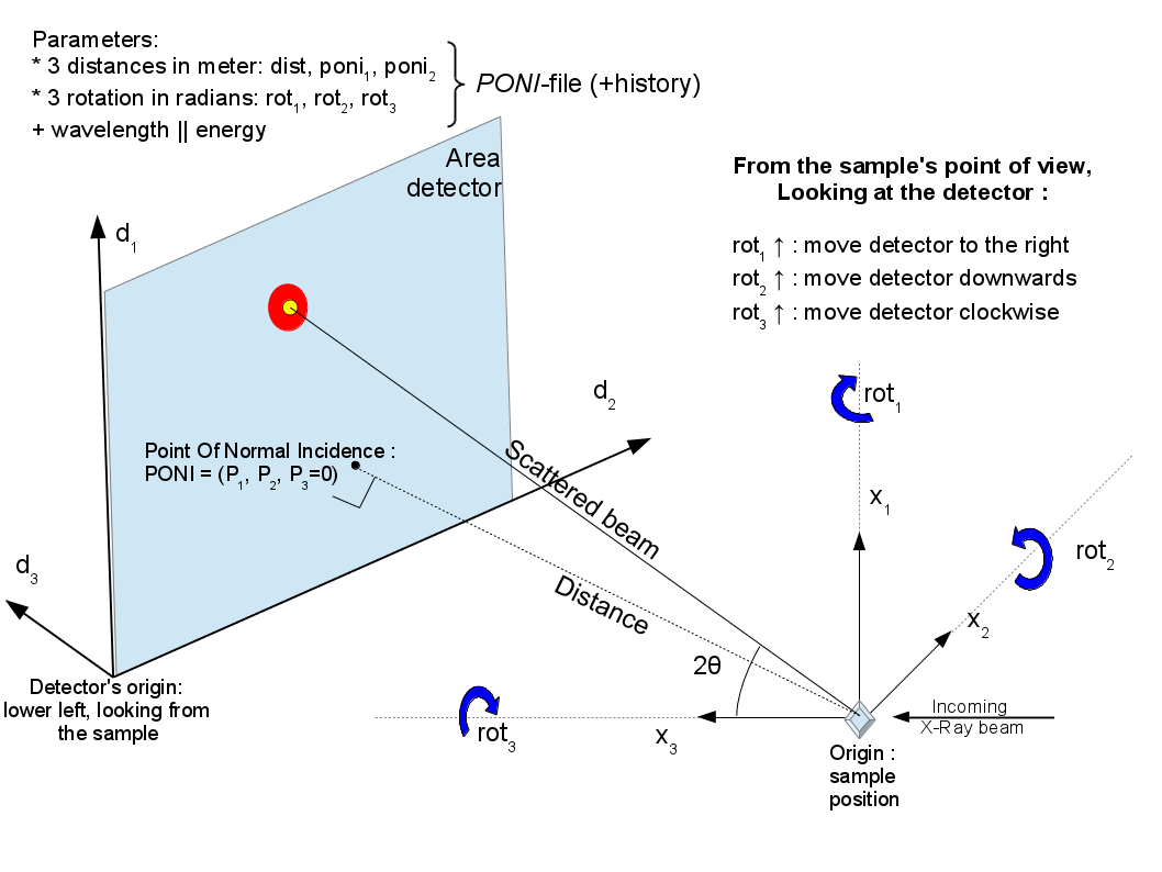
PONI figure

It may appear strange to have (x_1, x_2, x_3) indirect indirect but this has been made in such a way chi, the azimuthal angle, is 0 along x_2 and 90_deg along x_1 (and not vice-versa).

print("Processing time: %.3fs"%(time.time()-start_time))

Processing time: 7.502s