Geometries in pyFAI

This notebook demonstrates the different orientations of axes in the geometry used by pyFAI.

Demonstration

The tutorial uses the ipython notebook (aka Jupyter).

%pylab inline

Populating the interactive namespace from numpy and matplotlib

import pyFAI
from pyFAI.calibrant import ALL_CALIBRANTS

WARNING:pyFAI.utils:Exception No module named 'fftw3': FFTw3 not available. Falling back on Scipy

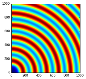
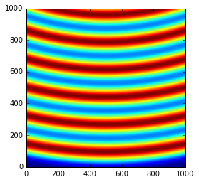
We will use a fake detector of 1000x1000 pixels of 100_µm each. The simulated beam has a wavelength of 0.1_nm and the calibrant chose is silver behenate which gives regularly spaced rings. The detector will originally be placed at 1_m from the sample.

wl = 1e-10
cal = ALL_CALIBRANTS["AgBh"]
cal.wavelength=wl

detector = pyFAI.detectors.Detector(100e-6, 100e-6)
detector.max_shape=(1000,1000)

ai = pyFAI.AzimuthalIntegrator(dist=1, detector=detector)
ai.wavelength = wl

img = cal.fake_calibration_image(ai)
imshow(img, origin="lower")

<matplotlib.image.AxesImage at 0x7f997becf7b8>

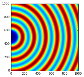
Translation orthogonal to the beam: poni1 and poni2

We will now set the first dimension (vertical) offset to the center of the detector: 100e-6 * 1000 / 2

p1 = 100e-6 * 1000 / 2
print(p1)
ai.poni1 = p1
img = cal.fake_calibration_image(ai)
imshow(img, origin="lower")

0.05

<matplotlib.image.AxesImage at 0x7f997ae09be0>

Let’s do the same in the second dimensions: along the horizontal axis

p2 = 100e-6 * 1000 / 2
print(p2)
ai.poni2 = p2
print(ai)
img = cal.fake_calibration_image(ai)
imshow(img, origin="lower")

0.05
Detector Detector    Spline= None    PixelSize= 1.000e-04, 1.000e-04 m
Wavelength= 1.000000e-10m
SampleDetDist= 1.000000e+00m        PONI= 5.000000e-02, 5.000000e-02m       rot1=0.000000  rot2= 0.000000  rot3= 0.000000 rad
DirectBeamDist= 1000.000mm  Center: x=500.000, y=500.000 pix        Tilt=0.000 deg  tiltPlanRotation= 0.000 deg

<matplotlib.image.AxesImage at 0x7f997ade7a20>

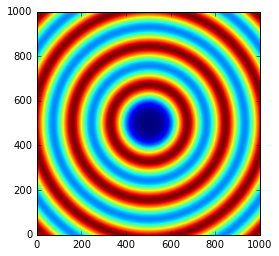
The image is now properly centered. We will now investigate the rotation along the different axes.

Investigation on the rotations:

Any rotations of the detector apply after the 3 translations (dist, poni1 and poni2)

The first axis is the vertical one and a rotation around it ellongates ellipses along the orthogonal axis:

rotation = +0.2
ai.rot1 = rotation
print(ai)
img = cal.fake_calibration_image(ai)
imshow(img, origin="lower")

Detector Detector    Spline= None    PixelSize= 1.000e-04, 1.000e-04 m
Wavelength= 1.000000e-10m
SampleDetDist= 1.000000e+00m        PONI= 5.000000e-02, 5.000000e-02m       rot1=0.200000  rot2= 0.000000  rot3= 0.000000 rad
DirectBeamDist= 1020.339mm  Center: x=-1527.100, y=500.000 pix      Tilt=11.459 deg  tiltPlanRotation= 180.000 deg

<matplotlib.image.AxesImage at 0x7f997ad42ef0>

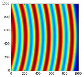
So a positive rot1 is equivalent to turning the detector to the right, around the sample position (where the observer is).

Let’s consider now the rotation along the horizontal axis, rot2:

rotation = +0.2
ai.rot1 = 0
ai.rot2 = rotation
print(ai)
img = cal.fake_calibration_image(ai)
imshow(img, origin="lower")

Detector Detector    Spline= None    PixelSize= 1.000e-04, 1.000e-04 m
Wavelength= 1.000000e-10m
SampleDetDist= 1.000000e+00m        PONI= 5.000000e-02, 5.000000e-02m       rot1=0.000000  rot2= 0.200000  rot3= 0.000000 rad
DirectBeamDist= 1020.339mm  Center: x=500.000, y=2527.100 pix       Tilt=11.459 deg  tiltPlanRotation= 90.000 deg

<matplotlib.image.AxesImage at 0x7f997ad26710>

So a positive rot2 is equivalent to turning the detector to the down, around the sample position (where the observer is).

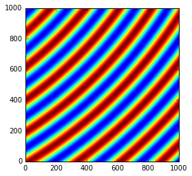
Now we can combine the two first rotations and check for the effect of the third rotation.

rotation = +0.2
ai.rot1 = rotation
ai.rot2 = rotation
ai.rot3 = 0
print(ai)
img = cal.fake_calibration_image(ai)
imshow(img, origin="lower")

Detector Detector    Spline= None    PixelSize= 1.000e-04, 1.000e-04 m
Wavelength= 1.000000e-10m
SampleDetDist= 1.000000e+00m        PONI= 5.000000e-02, 5.000000e-02m       rot1=0.200000  rot2= 0.200000  rot3= 0.000000 rad
DirectBeamDist= 1041.091mm  Center: x=-1527.100, y=2568.329 pix     Tilt=16.151 deg  tiltPlanRotation= 134.423 deg

<matplotlib.image.AxesImage at 0x7f997ac835c0>

rotation = +0.2
import copy
ai2 = copy.copy(ai)
ai2.rot1 = rotation
ai2.rot2 = rotation
ai2.rot3 = rotation
print(ai2)
img2 = cal.fake_calibration_image(ai2)
imshow(img2, origin="lower")

Detector Detector    Spline= None    PixelSize= 1.000e-04, 1.000e-04 m
Wavelength= 1.000000e-10m
SampleDetDist= 1.000000e+00m        PONI= 5.000000e-02, 5.000000e-02m       rot1=0.200000  rot2= 0.200000  rot3= 0.200000 rad
DirectBeamDist= 1041.091mm  Center: x=-1527.100, y=2568.329 pix     Tilt=16.151 deg  tiltPlanRotation= 134.423 deg

<matplotlib.image.AxesImage at 0x7f997ac63f60>

If one considers the rotation along the incident beam, there is no visible effect on the image as the image is invariant along this transformation.

To actually see the effect of this third rotation one needs to perform the azimuthal integration and display the result with properly labeled axes.

subplot(1,2,1)
I, tth, chi = ai.integrate2d(img, 300, 360, unit="2th_deg")
imshow(I, origin="lower", extent=[tth.min(), tth.max(), chi.min(), chi.max()], aspect="auto")
xlabel("2 theta (deg)")
ylabel("Chi (deg)")
subplot(1,2,2)
I, tth, chi = ai2.integrate2d(img2, 300, 360, unit="2th_deg")
imshow(I, origin="lower", extent=[tth.min(), tth.max(), chi.min(), chi.max()], aspect="auto")
xlabel("2 theta (deg)")
ylabel("Chi (deg)")

WARNING:pyFAI.geometry:No fast path for space: None
WARNING:pyFAI.geometry:No fast path for space: None

<matplotlib.text.Text at 0x7f997abd99e8>

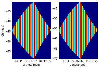
So the increasing rot3 creates more negative azimuthal angles: it is like rotating the detector clockwise around the incident beam.

Conclusion

All 3 translations and all 3 rotations can be summarized in the following figure:

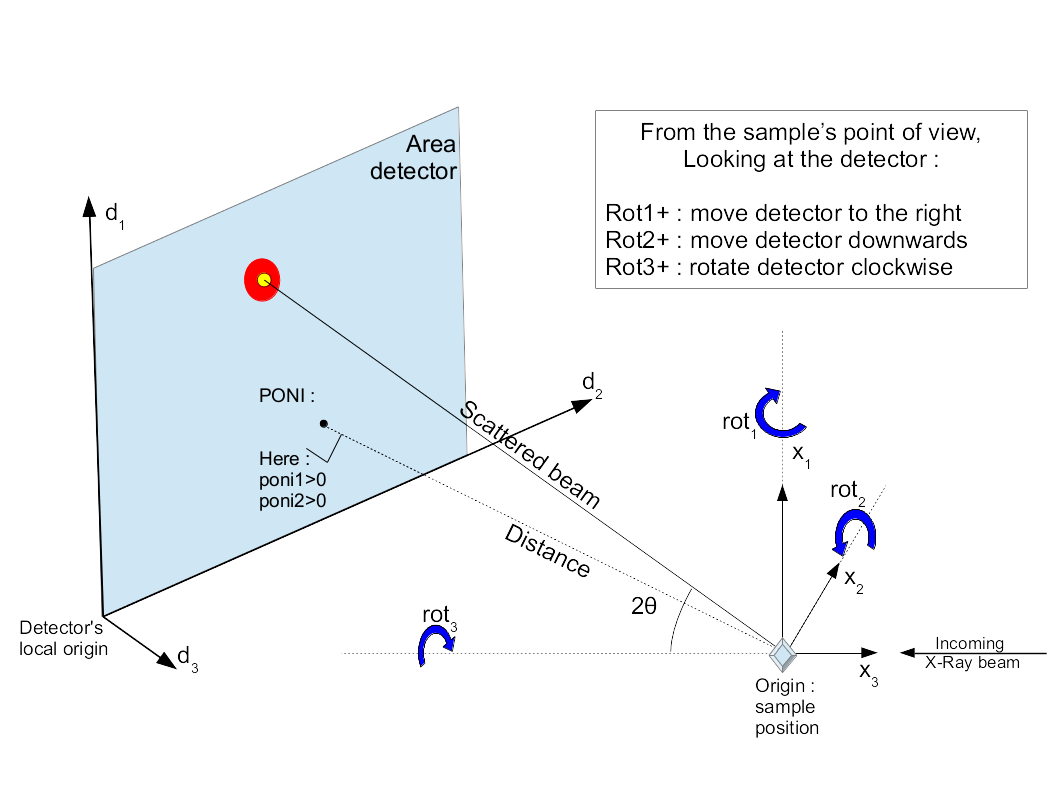
PONI figure

It may appear strange to have (x_1, x_2, x_3) indirect but this has been made in such a way chi, the azimuthal angle, is 0 along x_2 and 90_deg along x_1 (and not vice-versa).